Overlooked Details of BERT and Transformers

Introduction

Since the introduction of the Transformer model in “Attention is All You Need,” it has replaced RNNs/CNNs in various NLP tasks, becoming a new architecture for NLP. The original goal of the paper was to improve quality in translation tasks, but due to its outstanding performance, it has been applied to various language models and downstream tasks. It has also achieved impressive results in the visual domain.

This paper is written concisely and clearly, but due to space limitations, each sentence contains a large amount of information, making many details easy to overlook. Additionally, many design details are not proven by the authors but are based more on experience and intuition. After this paper, many works have attempted to further analyze Transformers.

This article collects and organizes some easily overlooked details (interview questions) in Transformers, mainly focusing on the Encoder part, for readers’ reference and study.

Table of Contents

Embedding

1. What is the difference between Position Encoding and Position Embedding?
2. Why does the Transformer multiply the Embedding at the end?
3. Why can the three Embeddings of BERT be added together?

Attention

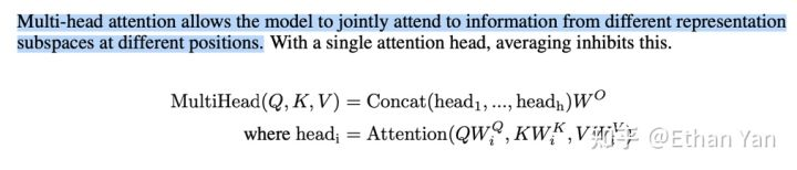
1. Why does the Transformer require Multi-head Attention?
2. Why do Q and K use different weight matrices in the Transformer?
3. Why do we need to divide before applying softmax?

LayerNorm

1. Why does the Transformer use LayerNorm instead of BatchNorm?

Q: What is the difference between Position Encoding and Position Embedding?

A: Position Embedding is learned, while Position Encoding is fixed.

The Transformer differs from RNNs/CNNs in that it does not contain sequence information. To incorporate sequence information, position encoding must be added. The paper mentions two encoding methods: learned and fixed.

Learned

The learned method is a straightforward scheme for position encoding, without any special design, directly treating position encoding as trainable parameters. For instance, if the maximum length is 512 and the encoding dimension is 768, a 512×768 matrix is initialized as the position vector, allowing it to be updated during training. Current models like BERT and GPT use this type of position encoding, which can actually be traced back further, as seen in Facebook’s “Convolutional Sequence to Sequence Learning” from 2017.

The general consensus is that a drawback of this learned absolute position encoding is that it is not scalable. If the pre-training maximum length is 512, it can only handle sentences of that length, and longer sentences cannot be processed.

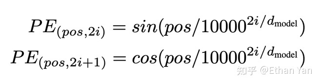
Fixed

Fixed position encoding is computed using trigonometric functions.

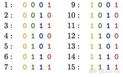
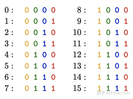
Why can periodic functions represent position encoding?

Refer to binary:

Another reason for using it is that it allows the model to easily learn relative positions.

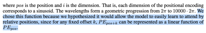
Because , this indicates that can be linearly represented.

Specifically, denote it as t.

Since k and t are constants, we can derive that can be linearly represented.

This is also why PE needs to use both sin and cos, rather than just one of them.

Why is there a magic number 10000 in the formula?

When i = 0, the period is , and when 2i = d_model = 512, the period is .

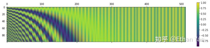
The following figure shows the changes of PE at different positions with different periods.

At 10000:

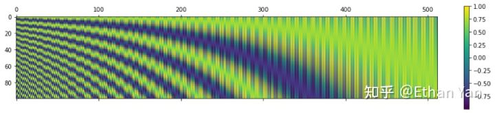
At 100:

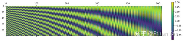
At 20:

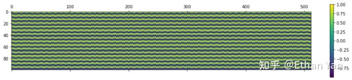
At 1:

Using 10000 is likely to ensure that the cycle period is large enough to encode sufficiently long texts.

For many techniques in deep learning, when you experiment enough, you will find that the only correct answer to these types of questions is: because experimental results show that this approach works better!

Experiments

Finally, the author tried both encoding methods (learned and fixed) and found that the results were quite similar.

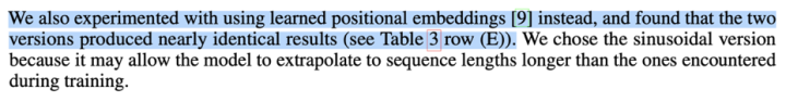
The experimental results are shown in the figure below:

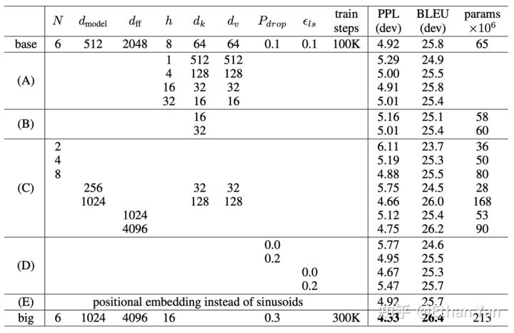
Row E shows the experimental results of the learned method, with PPL (the lower, the better) being the same as base, and BLEU (the higher, the better) being 0.1 lower. It can be seen that they are indeed quite similar. So why does BERT use the learned method? It may be because BERT’s training data is larger, allowing it to learn more, resulting in better experimental performance.

References

Su Jianlin. “Position Encoding in Transformer that Puzzles Researchers”: https://kexue.fm/archives/8130

Transformer Architecture: The Positional Encoding: https://kazemnejad.com/blog/transformer_architecture_positional_encoding/

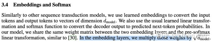
Q: Why does the Transformer multiply the Embedding at the end?

A: To make the scale of the embedding consistent with the position encoding.

Let’s first look at the original paper. The original paper only briefly mentioned this at the end, leaving the specific reason for readers to ponder.

Now looking at the code, indeed a constant needs to be multiplied during the forward pass.

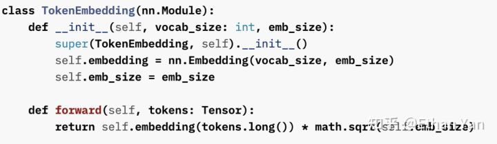
The specific reason is that if Xavier initialization is used, the variance of the embedding will be such that when it is very large, each value in the matrix will decrease. By multiplying by a constant, the variance can be restored to 1. The specific mathematical derivation is also quite simple and will be proven later when discussing scaled self-attention.

Since Position Encoding is calculated using trigonometric functions, its value range is [-1, 1]. Therefore, when adding Position Encoding, it is necessary to amplify the embedding values; otherwise, the inconsistent scales will lose information when added together.

Because BERT uses learned embedding, there is no need to amplify it here.

Q: Why can the three Embeddings of BERT be added together?

Explanation 1: Because adding the three embeddings is equivalent to concatenating the three original one-hot vectors and then passing them through a fully connected network. Compared to concatenation, addition saves model parameters.

Explanation 2: From the gradient perspective: (f + g + h)’ = f’ + g’ + h’

Reference: Why can the three Embeddings of BERT be added together?

https://www.zhihu.com/question/374835153

Sub-question: Why doesn’t BERT concatenate the three Embeddings?

Possible reason: it can be done, but it is unnecessary. Experiments show that addition performs better than concatenation; after concatenation, the dimension increases, requiring another linear transformation to reduce the dimension, which increases more parameters and is not worth the cost.

Additionally, addition can be seen as a special form of concatenation.

Reference: Why doesn’t BERT concatenate the three embedding vectors?

Zhihu https://www.zhihu.com/question/512549547

Q: Why does the Transformer require Multi-head Attention?

A: Experiments have shown that multi-head attention is necessary; using 8 or 16 heads can achieve better results, but using more than 16 heads can actually degrade performance. Each head focuses on different information, but the differences between heads decrease as the number of layers increases. Not all heads are useful; some works have attempted pruning to achieve better performance.

The paper mentions that the model is divided into multiple heads to form multiple subspaces, with each head focusing on different aspects of the information.

Subsequent research has also used visualization methods to analyze each head in each layer.

The figure shows that although many heads in the same layer exhibit similar patterns, there are still differences.

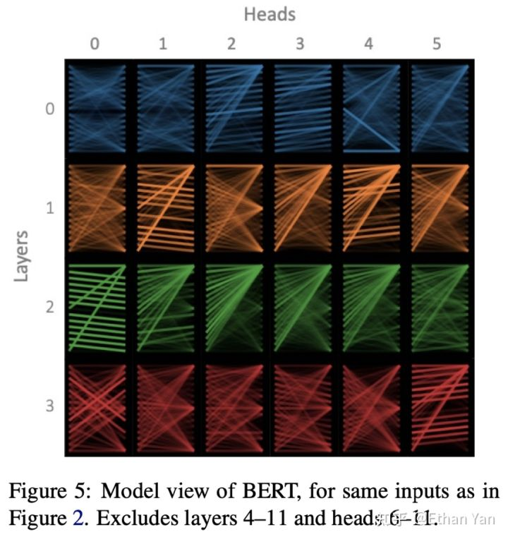
The figure indicates that the differences between heads decrease as the layer number increases. In other words, the variance between heads decreases as the layer number increases.

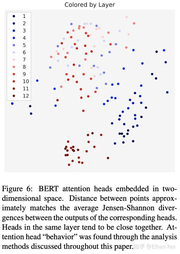
Different colors represent different layers, and the distribution of the same color indicates the differences among the heads in the same layer. We can first look at the first layer, which is deep blue. A point appears on the left, while points appear on the right and below, showing a sparse distribution. Now looking at the sixth layer, which is light blue, the distribution is relatively dense. Finally, in the twelfth layer, which is dark red, the points are almost entirely concentrated below, indicating a very dense distribution.

Some research has shown that some heads are actually not necessary; removing some heads still yields good results (and the decrease in performance may be due to the reduction in parameters). This is because with enough heads, these heads are already capable of focusing on position information and syntax information; adding more heads only serves to enhance or introduce noise.

Reference: https://www.zhihu.com/question/341222779/answer/814111138

Q: Why do Q and K use different weight matrices in the Transformer?

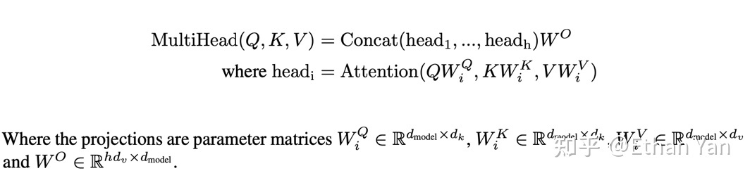
Q and K use different W_q and W_k to calculate, which can be understood as projections in different spaces. It is precisely due to this projection in different spaces that the expressive power is increased, allowing the resulting attention score matrix to have better generalization capabilities.

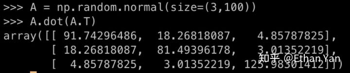
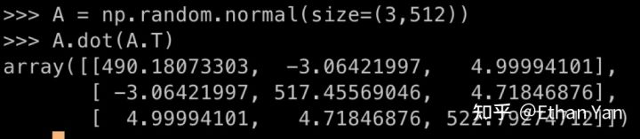
If the same W were used, the attention score would degenerate into an approximate diagonal matrix. This is because, before softmax, the diagonal elements are obtained by self-dot product, which results in a sum of many positive numbers, making them very large, while other elements have both positive and negative values, which are not as large. After softmax, the diagonal elements will approach 1.

An experiment was conducted to see what happens when a matrix is multiplied by its transpose. The diagonal elements are seen to be very large.

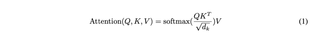
Q: Why do we need to divide before applying softmax?

A: To prevent gradient vanishing.

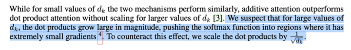
The explanation in the paper is that the dot product result of vectors will be large, pushing the softmax function into a region of very small gradients, and scaling will alleviate this phenomenon.

Why divide by , not some other number?

Regarding why the dimension affects the size of the dot product, the paper’s footnote actually provides some explanation:

Assuming vectors and have components , which are independent random variables with a mean of 0 and a variance of 1, then the mean of will be 0 and the variance will be .

To prove that the mean is 0:

To prove the variance is dk:

This uses a property of variance.

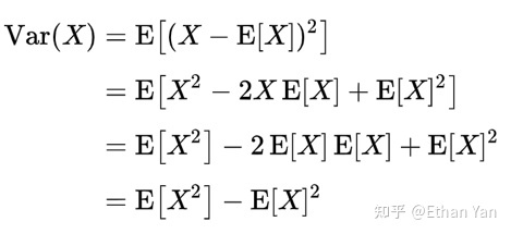
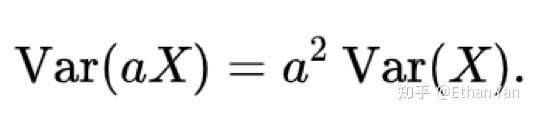
The scaled variance will return to 1:

This uses another property of variance:

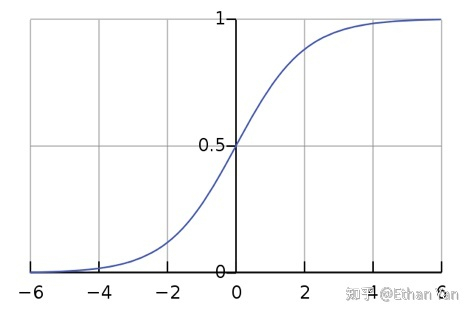
How to understand pushing the softmax function into a region of very small gradients?

The softmax function tends to learn to output 0 or 1. When the input is very small or very large, the output approaches 0 or 1, resulting in very small gradients.

This can also be understood from another angle: the sigmoid function is a special case of softmax. When the input is very large, the function enters a saturation region, resulting in very small gradients.

Here we directly provide the conclusion: when , the gradient with respect to is:

Expanding:

Based on the previous discussion, when the elements of the input are generally large, softmax will assign most of the probability distribution to the largest element, assuming our input is of large magnitude, resulting in a vector close to one-hot.

At this point, the above matrix becomes:

Where all gradients are close to 0.

Mathematical derivation process of softmax derivative: https://eli.thegreenplace.net/2016/the-softmax-function-and-its-derivative/

Thought 1: Does softmax + cross-entropy cause the gradient to vanish when inputs are too large/small?

No. Because cross-entropy has a log. The gradient of log_softmax is different from what was just calculated; even if one of the inputs x is too large, the gradient will not vanish.

Thought 2: What issues arise with softmax + MSE? Why don’t we use MSE as the loss function during classification?

The previous explanation can clarify this issue. Since MSE does not have a log, softmax + MSE will lead to vanishing gradients.

Q: Why does the Transformer use LayerNorm instead of BatchNorm?

Why normalize?

To stabilize the distribution of data and reduce the variance of the data. This transforms the data to have a mean of 0 and a variance of 1, preventing it from falling into the saturation region of the activation function, resulting in a smoother training process.

Why not use BatchNorm?

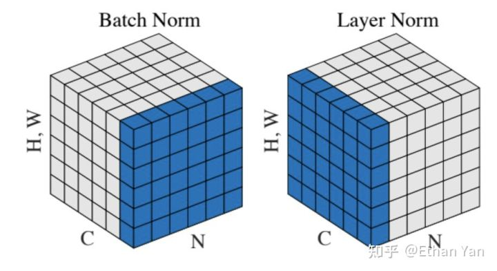
Different normalization methods operate on different dimensions. For images with dimensions [N, C, H, W]:

• BatchNorm computes statistics over the C dimension, flattening the differences within each C across (N, H, W).
• LayerNorm computes statistics over the N dimension, flattening the differences within each N across (C, H, W).

Note that this figure only illustrates examples in CV; in NLP, LayerNorm operates on:

• For input text with dimensions [N, L, E] (Batch size, sequence length, embedding size)
• Calculating statistics over (E) instead of (L, E).

From a data perspective: CV typically uses BatchNorm, while NLP usually employs LayerNorm. The correlation within a single channel of image data is relatively high, and the information across different channels needs to maintain diversity. In text data, the different samples within a batch are not highly correlated.

From the perspective of padding: different sentences have different lengths, and normalizing at the end of a sentence can be influenced by padding, making the statistics unreliable.

From a model perspective: In Self Attention, the upper bound of the size of the inner product is related to the L2Norm of q and k. LayerNorm directly restricts the L2Norm.

About Us