Mathematical Principles Behind Artificial Neural Networks

About 8000 words, recommended reading time 20 minutes.
This article introduces the mathematical principles behind artificial neural networks.

Introduction

When it comes to artificial intelligence algorithms, artificial neural networks (ANN) are an unavoidable topic. However, for beginners, it is often easy to be overwhelmed by the complex concepts and formulas in ANN, leading to a superficial understanding rather than a deep comprehension. Recently, the author has also been going through this painful process, and with the attitude that truth becomes clearer through discussion, I decided to sit down and carefully sort out these confusing issues to see if I could clarify the mathematical principles behind ANN.

In fact, the process of ANN is not very complex in summary. Taking the simplest feedforward neural network as an example, it is simply about:

Building the network architecture (with parameters to be determined)
Defining the loss function by comparing the output with the label (a function of the parameters to be determined)
Randomly providing a set of initial parameters
Providing a training sample (sgd) / a batch (Minibatch) (including the input and output values of ANN)
Forward propagation to obtain predicted labels and loss
Using gradient descent algorithm to adjust the network parameters from back to front (backpropagation, BP)
Obtaining all parameter values
Using the ANN

Among them, steps 4, 5, and 6 need to be iterated repeatedly (note that step 6 is a double loop).

Among the operations in ANN, the gradient descent algorithm is a relatively independent process, so let’s start with the gradient descent algorithm.

1. What Is Gradient Descent Actually Doing?

This question is actually very simple; people just get confused by the complex process of gradient descent and forget its essence. The gradient descent algorithm is always doing one thing — finding the extreme point of a function, and more precisely, the minimum point. However, this method is different from the classical methods we learned in higher mathematics for finding extreme points. So we must first ask, isn’t the classical method for finding extreme values good enough?

1.1 Finding Extreme Values: Isn’t the Traditional Method Good Enough?

To answer this question, let’s quickly review the traditional methods we learned in middle school and university for finding extreme points.

For a univariate function, extreme values may occur at points where the first derivative is zero (stationary points) or where the derivative does not exist.

For example, to find the extreme point of f(x) = x^2 + 3x:
Taking the derivative gives dy/dx = 2x + 3
Setting dy/dx = 0 gives x = -1.5 as a point where the derivative is zero.

Note that the point found above is only a possible extreme point, which is a necessary condition for the existence of extreme values. We also need to verify the sufficient condition to determine if it is indeed an extreme value. At this point, we can check the sign of the second derivative or determine the sign of the first derivative on both sides of the possible extreme point. Returning to our example:

When x < -1.5, 2x + 3 < 0
When x > -1.5, 2x + 3 > 0
This indicates that the function decreases around x = -1.5 and then increases,
therefore this point is a local minimum.

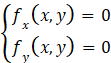
For a bivariate function, the situation is a bit more complex.First, we need to find the stationary points and points where the partial derivatives do not exist. These points are still only possible extreme points. The stationary points of a bivariate function need to satisfy the condition that both partial derivatives are zero, i.e.,

Mathematical Principles Behind Artificial Neural Networks

Clearly, finding the stationary points here requires solving a bivariate equation. We then need to find the values of its three second partial derivatives and use certain rules to determine whether they are extreme points.

It is also important to note that this judgment rule is different from that of univariate functions, because the sufficient condition for extreme values of univariate functions only requires examining one second partial derivative, while here we need to comprehensively examine three second partial derivatives of the bivariate function, which significantly increases the computational burden. Special treatment is also needed for cases where the partial derivatives do not exist.

In summary, we can see that while the classical method can accurately solve for extreme points, it is not practical when the number of variables in the function is large. For example:

This method lacks universality. By universality, we mean it cannot be easily generalized to multivariate cases. From the example of univariate to bivariate, we can see that with each additional variable, a new solution scheme must be studied. One can imagine that if it were a trivariate function, the number of second partial derivatives would be even greater, making the sufficient conditions for determining extreme values even more complex. ANN may need to solve for the extreme points of hundreds of millions of functions.
Secondly, this method requires solving a system of multivariate equations, and these equations are not necessarily linear. For such multivariate nonlinear equations, our intuitive feeling is that they are difficult to solve. In fact, although there are some numerical methods available for programming, the computational burden is high, and the solutions obtained are approximate, which has certain limitations.

Therefore, to find the extreme points of multivariate functions, we need to seek alternative methods. These methods should be simple and easy to implement, especially able to generalize easily to functions of any number of variables, and should also adapt to the characteristics of numerical computation in computers, as our program will certainly run on a computer. This is the so-called gradient descent algorithm.

1.2 What Is a Gradient?

The concept of a gradient is not difficult, but to ensure that as many people as possible understand it, let’s start with univariate functions. However, our goal now is to find the extreme values of a function using purely numerical methods, focusing only on the minimum values.

1.2.1 Finding Extreme Values of a Univariate Function: From Enumeration to Gradient Descent

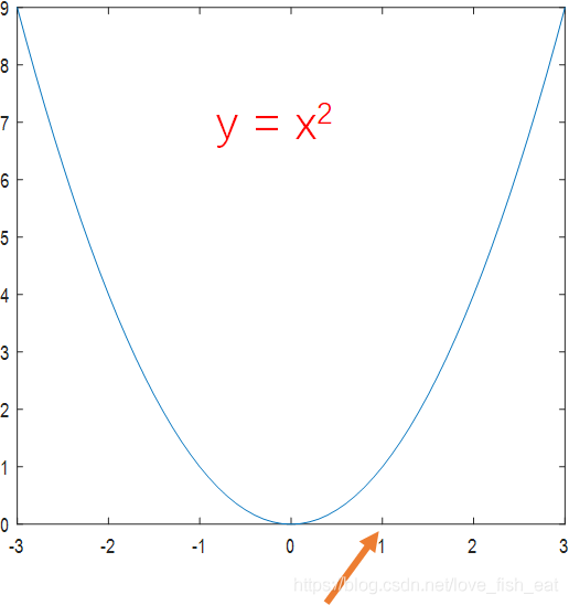
Let’s take a function as an example to see how to find extreme values.

Since we start from a certain point on the function, let’s imagine we are at x = 1. Is this point a local minimum? We can test it.

Move right 0.5, find f(1.5) > f(1), indicating this direction is increasing, so we should not choose this direction;
Move left 0.5, find f(0.5) < f(1), indicating this direction is decreasing, choose this direction;
Move left another 0.5, find f(0) < f(0.5), indicating this direction is decreasing, choose this direction;
Move left another 0.5, find f(-0.5) > f(0), indicating this direction is increasing, so we should not choose this direction.
Thus, we can take x = 0 as the local minimum.

Reviewing this process, we can abstract the process of finding local minimum points as follows:

First, choose a direction
Try taking a small step in that direction and determine if it is reasonable. If it is reasonable, take that step; if not, choose another direction.
Repeat the second step until you find the local minimum point.

Of course, there are a few points worth noting:

First, for a univariate function, we only have two options: moving left or moving right. In other words, at each step, our choice is limited and can be enumerated. Therefore, I call this method enumeration.
Second, we don’t need to trial and error to determine the direction; we can directly take the derivative. If the derivative value at a certain point is > 0, it indicates that the function is increasing at that point, and to find the local minimum, we should move left; conversely, if the derivative value < 0, we should move right.
Third, this method may not necessarily find the local minimum; whether it can find the extreme value is influenced by the chosen starting point and the step size taken each time.

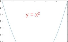
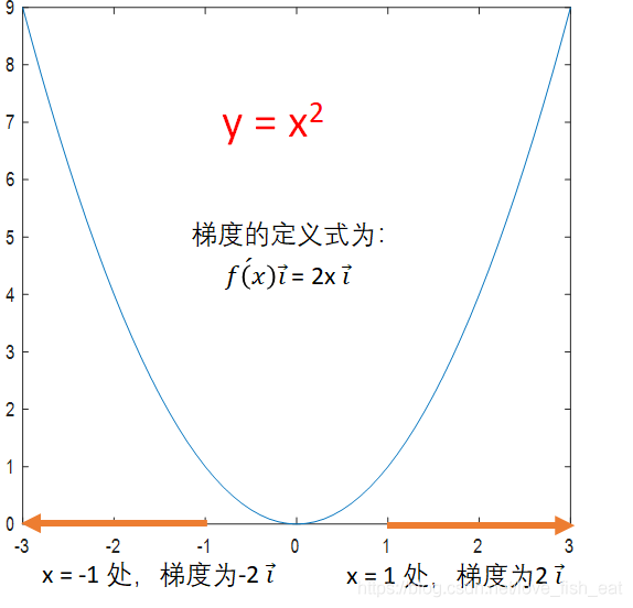
Regarding the second point, we can introduce the definition of a gradient.

A gradient is a vector that always points in the direction of the fastest increase of the function value. Its magnitude is the value of this fastest increase (the derivative). To obtain the gradient vector, it is simple; its components in the x, y, z… directions are just the corresponding derivative values. Thus, we can find the derivative.

For a univariate function, there are only two directions of change, and we define a one-dimensional vector to represent the gradient, such as 5i or -5i. When the number in front of i is positive, it indicates that the vector points in the positive direction of the x-axis; when negative, it indicates that the vector points in the negative direction of the x-axis. As shown in the figure below, the gradient vector defined in this way naturally points in the direction of function increase, isn’t it amazing?

Since the direction of the gradient is the direction of the fastest increase of the function, the opposite direction of the gradient becomes the direction of the fastest decrease of the function. Of course, for a univariate function, there is no concept of the fastest direction since there are only two directions to compare. However, with the gradient, we can further simplify the process of finding local minimum points:

First, calculate the gradient at a certain point
Move a small step in the opposite direction of the gradient
Repeat the first and second steps until you find the local minimum point.

Still taking the function as an example, starting point x = 1, let’s see how to find the extreme value using the gradient.

Initial x = 1, step size = 0.5
#In our example, the gradient calculation formula is 2xi. i is the unit vector pointing in the positive direction of the x-axis.
Calculating the gradient at x = 1 gives 2i, and the opposite gradient is -i #Note that here we only focus on the direction of the gradient; the magnitude of the gradient is not important.
Moving in this direction one step, x_new = x_old + step * coordinate of the negative gradient direction = 1 + 0.5 * (-1) = 0.5.
Calculating the gradient at x = 0.5 gives 1i, and the opposite gradient is -i.
Moving in this direction again, x_new = 0.5 - 0.5 * 1 = 0.
Calculating the gradient at x = 0 gives 0, indicating that we have reached the extreme point.

This is the process of using the gradient to find local minimum points, which is what the gradient descent algorithm does. It is not difficult to understand, right?

As we can see, compared to enumeration, the gradient descent method is much more intelligent; it directly gives the correct direction without needing us to test step by step. Furthermore, using the gradient descent method does not require us to focus on specific function values; we only need to pay attention to the derivatives, and we only need to consider the first derivative.

Later, we will give the step size mentioned above a more sophisticated name — learning rate, which is the terminology used in machine learning.

In this context, I have normalized the gradient, but it is also possible not to do so. This way, when the function changes dramatically, the distance moved will be larger; when the function changes more gently, the distance moved will be shorter. For example, in our case, we could reach the result in just one iteration.

Initial x = 1, learning rate = 0.5
#In our example, the gradient calculation formula is 2xi. i is the unit vector pointing in the positive direction of the x-axis.
Calculating the gradient at x = 1 gives 2i, and the opposite gradient is -2i #Note that here we are concerned with both the direction of the gradient and its magnitude.
Moving in this direction one step, x_new = x_old + step * negative gradient coordinate = 1 + 0.5 * (-2) = 0.
Calculating the gradient at x = 0 gives 0, indicating that we have reached the extreme point.

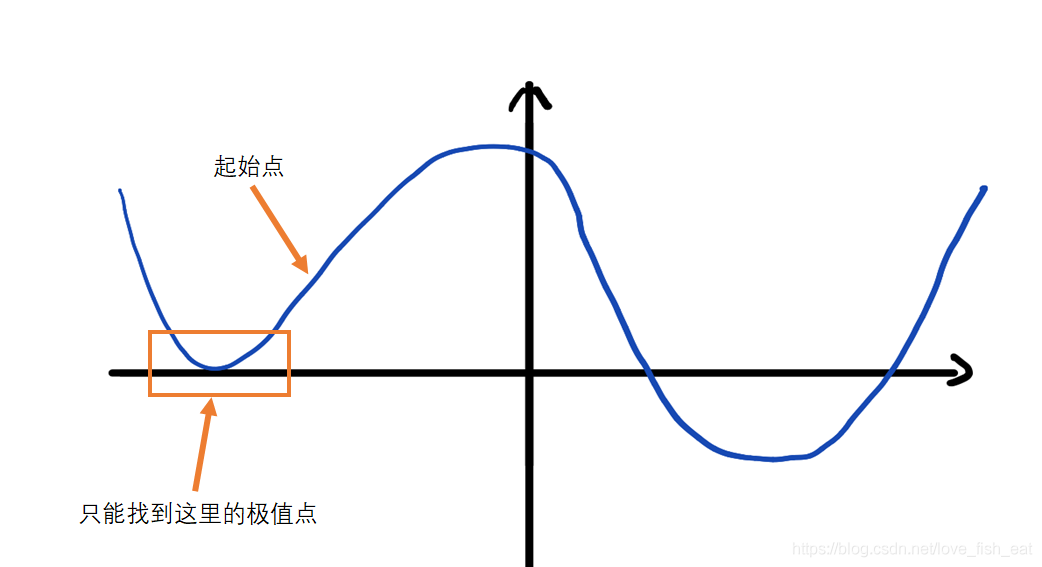
Now that we have discussed gradients, let’s address the third point mentioned earlier about not being able to find extreme values by giving two specific examples.

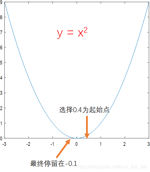
Consider the function, if the starting point is chosen as 0.4, while keeping the learning rate at 0.5, it cannot find the actual local minimum.

In this case, we can achieve more precise results by reducing the learning rate; for example, setting the learning rate to 0.1 will still yield accurate results. In practice, the learning rate is generally set to 0.1.

For functions that have multiple extreme points, this method cannot find all extreme points, let alone the global extreme point. In this case, we can introduce some randomness into the algorithm to have a certain probability of escaping local extreme points.

1.2.2 Gradient of Multivariate Functions

As mentioned earlier, one of the advantages of the gradient descent algorithm is its ease of generalization to multivariate functions. Now let’s take a bivariate function as an example to see how the gradient helps us find extreme points.

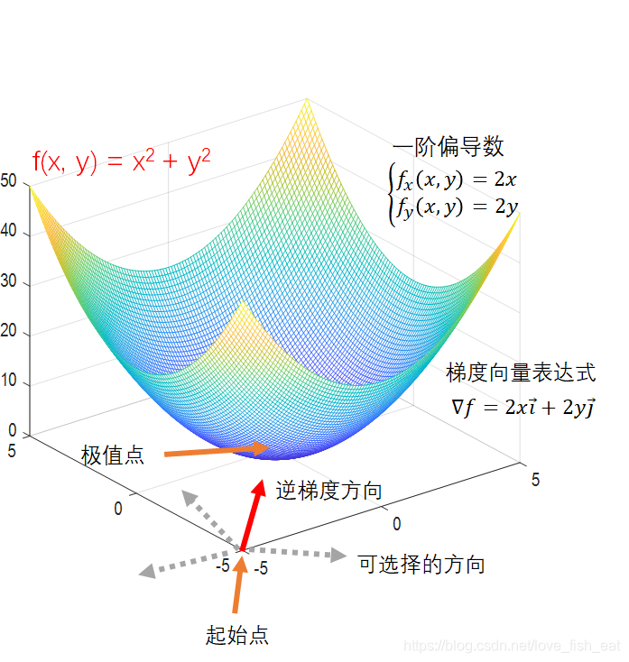
This time, our function changes, and we choose the starting point as (-5, -5), with the learning rate still set at 0.5. Our goal is to find the extreme point of this function, which we know should be (0, 0).

There are a few differences compared to univariate functions:

First, a bivariate function describes the relationship between one independent variable and two dependent variables, meaning the domain of the function is a two-dimensional plane, and the extreme point we are looking for lies on this two-dimensional plane.
Secondly, since we are searching for extreme points on a two-dimensional plane, the directions we can choose at each step are no longer limited to left or right, but rather an infinite number of directions. Therefore, the enumeration method is completely ineffective. Fortunately, we have the more intelligent gradient descent method.
The derivative in the univariate gradient definition now changes to partial derivatives of multivariate functions.

Now, let’s begin the algorithm:

Starting point coordinates (-5,-5), learning rate = 0.5
#In our example, the gradient calculation formula is 2xi + 2yj. i and j are unit vectors pointing in the positive directions of the x and y axes respectively.
Calculating the gradient at point (-5,-5) gives -10i-10j, and the negative gradient is 10i+10j, written in coordinate form as (10,10).
At point (-5,-5), move one step along this gradient.

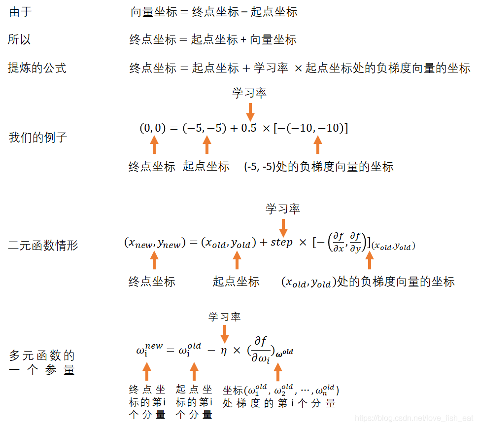
Using the formula: vector coordinates = endpoint coordinates - starting point coordinates, we get the endpoint coordinates = starting point coordinates + vector coordinates.

Here, the endpoint coordinates are (x_new, y_new), starting point coordinates are (x_old, y_old) = (-5, -5), and vector coordinates are negative gradient coordinates = (10,10). Considering the learning rate, we can obtain:
(x_new, y_new) = (-5, -5) + 0.5 * (10, 10) = (0, 0).

Calculating the gradient at (0, 0) gives the zero vector, indicating that we have reached the extreme point.

By abstracting the above process, we have obtained the complete logic of the gradient descent algorithm:

We want to find the extreme minimum points of the function (the set of independent variables that minimize the function value), because the direction of the gradient is the direction of the fastest increase of the function value, so moving in the opposite direction of the gradient results in the fastest decrease of the function value.

Thus, as long as we move step by step in the opposite direction of the gradient, we can approach the set of independent variable values that minimize the function value.

How do we move step by step in the opposite direction of the gradient?

We randomly specify a starting point (a set of independent variable values) and then compute the unknown endpoint coordinates along the direction of the gradient. The gradient is a vector and also has coordinates.

Through the iterative formula above, regardless of how many variables the function has, each of its independent variables will quickly approach the extreme point (or its approximation). Thus, we can find a set of independent variable values that minimize the function value as much as possible.

1.2.3 Summary

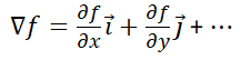
The gradient calculation formula is
A gradient is a vector that always points in the direction of the fastest increase of the function value, and its magnitude is the value of this fastest increase (the derivative).
The gradient descent method is a method for numerically solving the extreme points of a function.
Its process can be summarized as gradually approaching the possible extreme points along the opposite direction of the gradient.
The reason for using gradient descent is that other methods for finding extreme points (such as traditional methods, enumeration) lack computability and cannot be implemented in programming.
The gradient descent method can easily be generalized to multivariate functions, making it suitable for programming.
Remember that in this process, we are looking for extreme points (the set of independent variables that minimize the function value) rather than the specific extreme value.
The disadvantage of gradient descent is that it may not find the global optimal solution.

2. Artificial Neural Networks (ANN)

If you are hearing the term artificial neural networks for the first time, you might feel it sounds quite grand, as if we can already mimic the mysterious nervous system. In fact, it is just a mathematical model. Of course, the effects of ANN are impressive, making it seem like computers suddenly have human-like capabilities, such as recognizing people and objects.

However, upon further abstraction, we can realize that it is merely a classifier. Its input is an image, or more precisely, a set of numerical values representing pixel points, and its output is a category.

In simple terms, the so-called artificial neural network is essentially a very large function.

This is akin to the relationship between airplanes and birds. The reason an airplane can fly is not because we imitate a bird, but because we build a mathematical model based on principles in fluid mechanics, then calculate the dimensions and shape of the airplane and design the corresponding engine.

2.1 Mathematical Model of Neurons

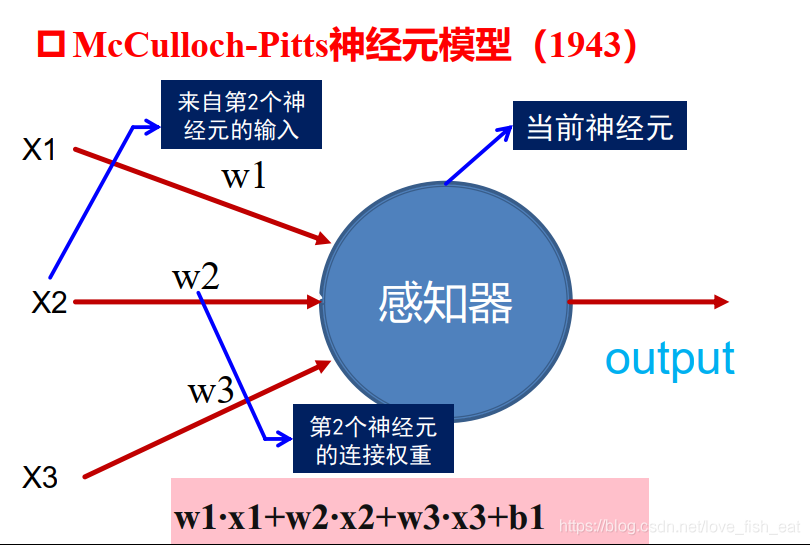
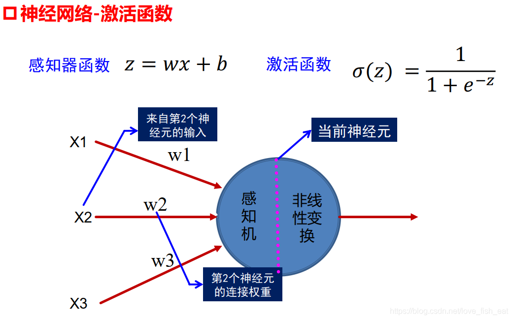
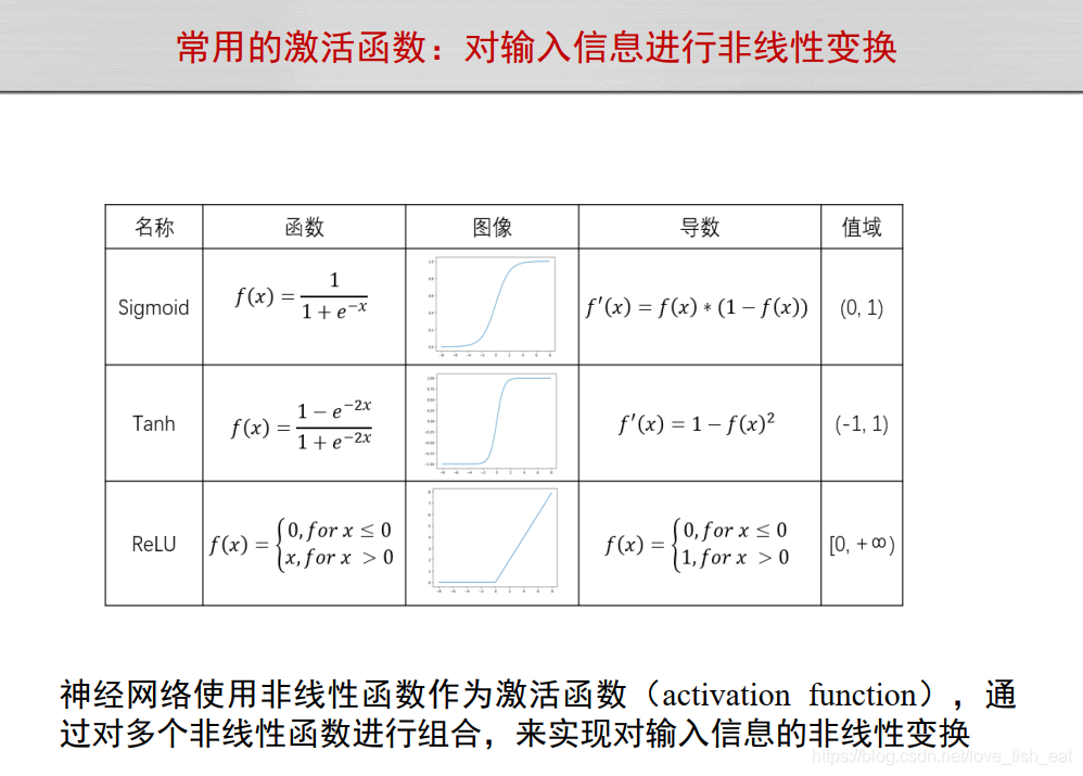
To illustrate the issue, let’s borrow a diagram from a teacher’s PPT. We can see that each node in an ANN (also known as a neuron) is a simple linear function model.

Of course, we can introduce some non-linear factors through activation functions to enhance the model’s expressive power. In this case, the neuron below represents such a function,

where w1, w2, w3, and b are parameters, and x1, x2, x3 are the function’s inputs, i.e., the dependent variables.

Common activation functions are shown here (still borrowing from the teacher’s PPT, covering face and escaping~).

The above is what is called an artificial neuron or artificial neuron. Many such neurons connected according to certain rules constitute ANN, which is why I said ANN is just a very large function.

Is it quite different from the grand neurons you imagined? However, the so-called artificial intelligence we have today is merely such a mathematical model. Whether it is a simple image classifier or the AlphaGo that defeated humans, it all relies on such mathematical calculations to derive results, rather than some magical power.

2.2 How Is ANN Created?

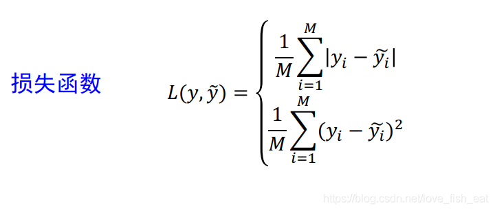
Now that we understand the essence of ANN, let’s see what needs to be done to obtain an ANN. Here, please pay attention as we will encounter functions with different functionalities, and do not confuse them.

Since ANN is a very large function, the first thing we do is build the architecture of this function, that is, design the architecture of the artificial neural network. At this point, this function has a bunch of parameters that need to be determined. Next, we prepare a bunch of training data to train the ANN, which means determining all the parameters mentioned above. The model is complete and can be used.

Clearly, the most critical step is the third step — determining the unknown parameters.

First, let’s explain training data. We know that ANN is a classifier and also a function. This function reads some input values, and after complex calculations, it outputs values that can be interpreted as categories. The training data consists of a set of data where both the input values and the final output values are known, in other words, it is a known correspondence between a set of independent variable values and dependent variable values.

To put it more clearly, our task is to find the unknown parameters of the function, given the architecture of the function and a set of input and output values. I refer to this function we want to derive as the target function. Thus, in summary, our task is to find the unknown parameters of the target function.

To accomplish this task, we introduce another important concept — the loss function.

2.2.1 Loss Function

Here, we will play a little trick. Pay attention, this is very critical!!!

Since we know a set of inputs and outputs for the target function, and we do not know its parameters, let’s treat these unknown parameters as dependent variables and directly substitute the inputs into the target function. This way, we get a function where the independent variable is the unknown parameters of the target function and the function itself is completely known.

At this point, if we can find a suitable set of unknown parameters, this function should output values that are completely consistent with the known inputs.

Thus, we can define the loss function by calculating the difference.

The above figure shows two forms of the loss function (in addition to which there are cross-entropy loss functions and other types). Generally, we need to choose an appropriate loss function based on different task types. To facilitate beginner understanding, the subsequent discussion will use the second form, mean squared error. The summation symbol appears here because the output end of ANN may correspond to more than one function, and these functions can represent the probabilities of categorizing an image into different classes. We will introduce an intuitive example later, which will be self-evident.

It is important to note that while the loss function still seems to have the shadow of the target function, it is actually completely different. Let’s compare them in a table:

Target Function	Loss Function
Expression	f	loss
Generation Method	Pre-constructed framework, then derive the parameters through training	Compare the output of the target function with the actual value to obtain the framework, then substitute a specific training sample (including input values and label values)
Independent Variables	—— Input values of the neural network (in practical situations, this can be all pixel values of an image)	—— Unknown parameters of the target function
Function Value (Dependent Variable) Meaning	Probabilities belonging to different categories	Difference between predicted value and actual value (the smaller, the better)
Characteristics	The function we ultimately want to obtain can be used for image classification. It is a combination of linear and nonlinear functions, large scale, with many independent variables and parameters	Used to derive the transitional function of the target function. Non-negative, with a minimum value of 0, generally requires using gradient descent to find the extreme point.

Let’s look at an example to see the process of function transformation. Assume the original function is a bivariate function of the form, where a, b, and c are constants or unknown parameters. Now we provide a set of specific input values, for example, substituting them into the function and treating a, b, and c as variables, the function transforms into a trivariate function, denoted as.

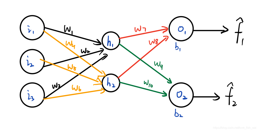
In summary, the process of finding the target function has transformed into the process of finding the extreme points of the loss function, and isn’t finding the extreme points what we can achieve using the gradient descent method introduced above?

2.2.2 An Example: Chain Rule Derivation and Backpropagation (BP)

Up to this point, we have covered important concepts related to ANN, but we have yet to mention chain rule derivation and backpropagation (BP). Let’s use an example to integrate everything.

Consider the following simple ANN:

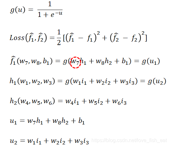
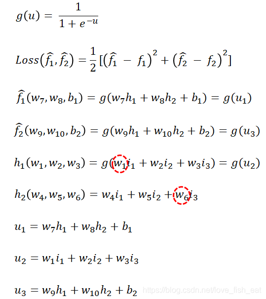
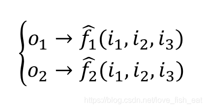
This ANN has four neurons, which are. It outputs two target functions, both of which are functions of the input variables, denoted as

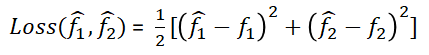
Now we define the loss function as

Note that we will now substitute a specific set of input variables, making the loss function a fully determined function without unknown parameters (the specific process of variable change is referenced in the previous description). Here, is a middle variable, and they are all multivariate functions of one variable.

Now, as long as we provide a training sample containing input and output data, the loss function becomes a completely determined function without unknown parameters. Our task is to find the extreme points of this loss function.

According to the derivation of the gradient descent algorithm, we can find this extreme point by following these steps:

Randomly specify a set of initial parameters
Calculate the partial derivatives of the Loss function with respect to each parameter. Note that this step requires substituting specific values for the parameters, meaning this step yields a numerical result.
Update each parameter value according to the gradient descent formula until certain conditions are met.

Steps 2 and 3 need to be iterated repeatedly.

Now, let’s take a look at how to adjust a few of the parameters during the adjustment process.

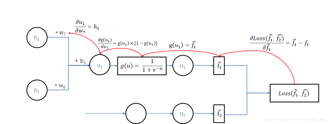
Let’s try adjusting; we need to calculate the partial derivative of the loss function with respect to the variable (note that this is a numerical value, not an expression), so let’s write out its dependency relationship:

Here, the Loss function depends on the variable , but not on . When deriving the function with respect to , we should treat as a constant.

Thus, the result of the derivative is

In fact, it is clear from the neural network diagram where the derivatives are derived.

Here are a few key points:

First, each term in the equation is indexed with w, indicating that specific values will be substituted into the equation to yield a numerical result.
Secondly, when g(u) represents the sigmoid function, the derivative result is
When calculating the partial derivative of the function with respect to a variable, it is also a function, but it is a function of independent variables and should be treated as a constant. Thus, the result of the partial derivative is
The last three terms on the right side of the equation can be independently calculated once a training sample is provided and initial parameters are specified.

Once we obtain the numerical value of the partial derivative of the loss function with respect to , we can adjust this parameter according to the formula derived from the gradient descent algorithm!

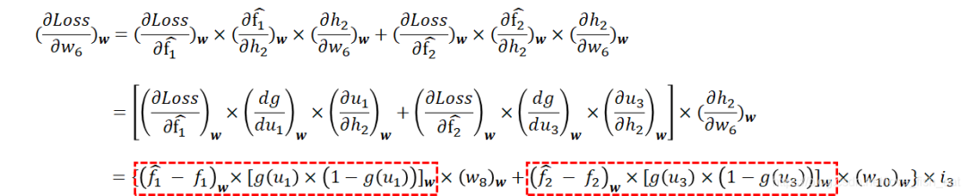
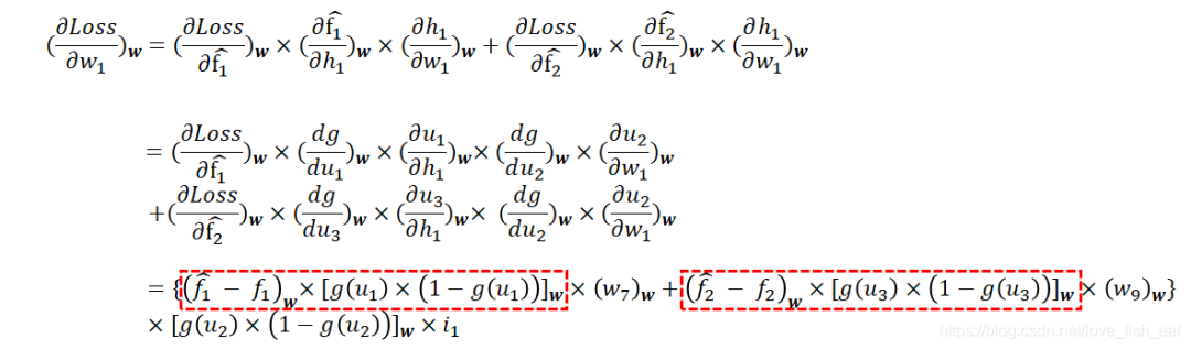
It can be seen that and are variables of functions and, and both functions depend on and, so the loss function needs to take partial derivatives with respect to both.

We again apply the chain rule to derive the partial derivatives:

For the partial derivative, we have:

Notice that the part circled in red looks somewhat familiar, doesn’t it?

In fact, this part has already been calculated when adjusting the parameters of the previous layer (please refer back to the calculation formula). Therefore, in programming, we can save intermediate results so that we can reuse them here.

Now, looking at the entire process, we are amazed to discover that for ANN, when we need to use it, we start by providing input and then calculate the output of this large and complex function step by step; when we need to train it, we start from the parameters at the end and calculate the derivatives step by step, adjusting each parameter. Moreover, calculating the previous parameters usually involves using previously computed intermediate results.

Thus, the process of adjusting parameters in ANN can be seen as a process of backpropagation (BP).

The reason for this backpropagation is that the parameters at the back of the neural network depend on fewer intermediate variables and have fewer composite layers, while the parameters at the front have undergone multiple composites, resulting in a long chain of derivatives.

2.2.3 One Last Small Issue

Above, we went through the entire process of calculating partial derivatives, but calculating partial derivatives is just one part of the gradient descent algorithm.

Once the program runs, we will calculate the partial derivatives for each training sample repeatedly until we find the extreme point.

This means that according to the gradient descent algorithm, each training sample will ultimately yield a set of parameter values.

Clearly, a training set will contain multiple training samples, so we will end up with many different sets of parameter values.

However, the training goal of ANN is to determine a set of parameter values to obtain a complex function with a certain effectiveness.

How to Solve This?

For each parameter, we can average the different values obtained from different training samples. Alternatively, we can construct a larger loss function, i.e., summing the loss functions generated by each training sample and then using gradient descent to find the extreme point of this cumulative loss function.

In this way, we can ultimately determine all the parameters of the ANN through training and then use it to perform some magical tasks.

Editor: Wang Jing

Proofreader: Yang Xuejun

1.1 Finding Extreme Values: Isn’t the Traditional Method Good Enough?

1.2 What Is a Gradient?

2.1 Mathematical Model of Neurons

2.2 How Is ANN Created?

Leave a Comment Cancel reply