Recently, the Google Translate that has been spreading like wildfire among friends has achieved stunning performance. The core technology here is RNN – the so-called Recurrent Neural Network. RNN can be regarded as one of the most promising tools in deep learning’s future. Do you want to understand the source of its power? Do you want to know some of the latest applications of RNN? Please see below.
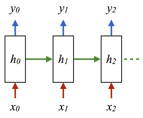
Why does RNN have such powerful effectiveness? Let’s start from the basics. First, we need to look at the structural differences between RNN and convolutional networks (CNN), which have established great achievements in processing static variables like images. The term “recurrent” already points out the core feature of RNN, which is that the system’s output is retained in the network and jointly determines the next output along with the system’s input at the next moment. This embodies the essence of dynamics, as the recurrence corresponds to the feedback concept of dynamic systems, capable of depicting complex historical dependencies. From another perspective, it also aligns with the famous Turing machine principle.
At this moment, the state contains the history of the previous moment and serves as the basis for the changes at the next moment. This actually contains the core concept of programmable neural networks, namely, when you have an unknown process but can measure the input and output, you assume that when this process passes through RNN, it can learn the input-output patterns by itself and thus has predictive capabilities. In this respect, RNN is Turing complete.

Figure: Figure 1 is the architecture of CNN, Figures 2 to 5 are several basic applications of RNN. Figure 2 transforms a single input into a sequence output, such as converting an image into a line of text. Figure 3 converts a sequence input into a single output, like sentiment analysis, measuring whether a piece of text has positive or negative emotions. Figure 4 converts a sequence into a sequence, the most typical being machine translation, noting the “time difference” between input and output. Figure 5 is a conversion from sequence to sequence without time difference, such as labeling each frame in a video. Image source: The Unreasonable Effectiveness of RNN.
Let’s use a small piece of Python code to help you understand the principles mentioned above:
class RNN:
# …
def step(self, x):
# update the hidden state
self.h = np.tanh(np.dot(self.W_hh, self.h) + np.dot(self.W_xh, x))
# compute the output vector
y = np.dot(self.W_hy, self.h)
return y
Here, h is the hidden variable, i.e., the state of each neuron in the entire network, x is the input, and y is the output. Note that all three are high-dimensional vectors. The hidden variable h is what we usually refer to as the essence of the neural network, and it is the basis for the recurrence because it acts like a reservoir that can theoretically store infinite historical information. On one hand, it absorbs the current value of the input sequence x through the input matrix W_xh, and on the other hand, it interacts with other internal neurons through the network connection W_hh (network effects, information transmission), because its network state is related to the entire past history of inputs, and the final output is the sum of both parts passed through the nonlinear function tanh. The entire process is the “recurrence” process of a recurrent neural network. The W_hh can theoretically depict any feedback form of the entire history of inputs on the final output, which is the key to RNN’s power.

Then, it seems that CNN also has similar functions? Can CNN be used as RNN? The answer is no. The important feature of RNN is its ability to handle inputs of variable lengths and produce consistent outputs. When your inputs can be of varying lengths, such as when training translation models, where the lengths of sentences are not fixed, you cannot use CNN, which is trained on fixed-pixel images, to handle this. However, the recurrent characteristics of RNN can easily manage this.
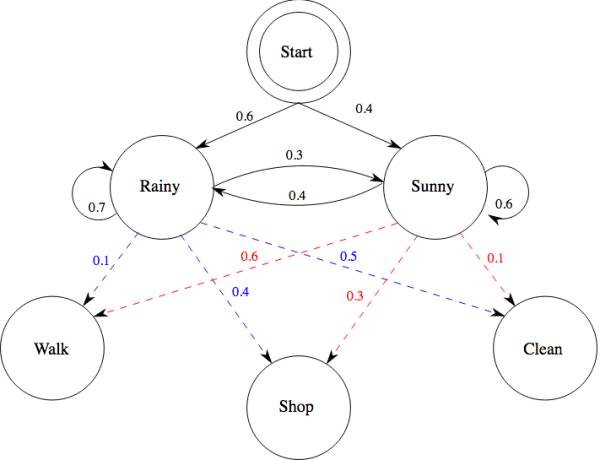
The essence of RNN is a data inference machine. It can find associations between two time series, and as long as there is enough data, it can obtain the probability distribution function from x(t) to y(t), thus achieving inference and prediction. Here, we undoubtedly recall another powerful tool for time series inference – HMM, the Hidden Markov Model, where there is also an input x, an output y, and a hidden variable h. The difference between h in this model and h in RNN is the iterative rule; the hidden variable is linked to the next hidden variable through a transition matrix. The transition matrix changes over time, while RNN does not have the concept of a transition matrix, but instead has a connection matrix between neurons. HMM is essentially a Bayesian network, so each node has actual meaning, whereas the neurons in RNN are merely hubs for information flow, without actual corresponding meanings. There are still intricate connections between the two.
First, the tasks that HMM can accomplish, RNN can almost also do, such as language modeling, but RNN’s dimensions will be higher. In these tasks, RNN effectively expresses the transition matrix of HMM through its network. In terms of training methods, HMM can derive the most likely values of hidden variables and transition matrices through algorithms similar to EM for maximum posterior probability. RNN can be trained through general gradient backpropagation algorithms.

Now, let’s look at some specific cases of RNN handling tasks:
For example, learning to speak! How do we make a computer produce something resembling human speech?
Here we start from a very specific program, showing you how to design a program step by step to perform the simplest language generation task, which aims to make the neural network play a word game, where it guesses the next letter after being given a letter, for example, give it ‘Hell’, and it follows with ‘o’. The diagram is as follows:
data = open(‘input.txt’, ‘rw’).read() # should be simple plain text file
chars = list(set(data)) # vocabulary
data_size, vocab_size = len(data), len(chars)
print ‘data has %d characters, %d unique.’ % (data_size, vocab_size)
char_to_ix = { ch:i for i,ch in enumerate(chars) } # vocabulary
ix_to_char = { i:ch for i,ch in enumerate(chars) } # index
First, we express the letters as vectors, using a function called enumerate, which is like building a digital dictionary (vocabulary) for the language. After this step, the language information is transformed into a digital time series.
hidden_size = 100 # size of hidden layer of neurons
seq_length = 25 # number of steps to unroll the RNN for
learning_rate = 1e-1
# model parameters
Wxh = np.random.randn(hidden_size, vocab_size)*0.01 # input to hidden
Whh = np.random.randn(hidden_size, hidden_size)*0.01 # hidden to hidden
Why = np.random.randn(vocab_size, hidden_size)*0.01 # hidden to output
bh = np.zeros((hidden_size, 1)) # hidden bias
by = np.zeros((vocab_size, 1)) # output bias
Next, we need to initialize three matrices, namely W_xh, W_hh, and W_hy, which represent the connections between the input and the hidden layer, the hidden layer and itself, and the hidden layer and the output, as well as the biases (bh and by) in the activation function of the hidden layer and output layer:
Loss=[ ]
Out=[ ]
while True:
# prepare inputs (we’re sweeping from left to right in steps seq_length long)
if p+seq_length+1 >= len(data) or n == 0:
hprev = np.zeros((hidden_size,1)) # reset RNN memory
p = 0 # go from start of data
inputs = [char_to_ix[ch] for ch in data[p:p+seq_length]]
targets = [char_to_ix[ch] for ch in data[p+1:p+seq_length+1]]
The next step is to start the program, first preparing the input:
# sample from the model now and then
if n % 100 == 0:
sample_ix = sample(hprev, inputs[0], 200)
txt = ‘ ‘.join(ix_to_char[ix] for ix in sample_ix)
print ‘—-
%s
—-‘ % (txt, )
This step involves checking the results every hundred iterations to see if the sentences generated by the RNN are becoming more human-like. Sampling means giving it a starting letter, and then the neural network outputs the next letter, which together serves as input for the next letter, and so on:
# forward seq_length characters through the net and fetch gradient
loss, dWxh, dWhh, dWhy, dbh, dby, hprev, y = lossFun(inputs, targets, hprev)
smooth_loss = smooth_loss * 0.999 + loss * 0.001
if n % 100 == 0: print ‘iter %d, loss: %f’ % (n, smooth_loss) # print progress
This step is about finding the gradient; the loss function calculates the gradient, and the key is measuring the information returned for learning. The content of the function will be released at the end.
Finally, we adjust the values of the parameters based on the gradient, which is the learning process.
# perform parameter update with Adagrad
for param, dparam, mem in zip([Wxh, Whh, Why, bh, by], [dWxh, dWhh, dWhy, dbh, dby], [mWxh, mWhh, mWhy, mbh, mby]):
mem += dparam * dparam
param += -learning_rate * dparam / np.sqrt(mem + 1e-8) # adagrad update
p += seq_length # move data pointer
n += 1 # iteration counter
Loss.append(loss)
Out.append(txt)
This is the main program; yes, it’s that simple. The loss function that was just omitted is as follows:
def lossFun(inputs, targets, hprev):
“””
inputs, targets are both lists of integers.
hprev is Hx1 array of initial hidden state
returns the loss, gradients on model parameters, and last hidden state
“””
xs, hs, ys, ps = {}
hs[-1] = np.copy(hprev)
loss = 0
# forward pass
for t in xrange(len(inputs)):
xs[t] = np.zeros((vocab_size,1)) # encode in 1-of-k representation
xs[t][inputs[t]] = 1
hs[t] = np.tanh(np.dot(Wxh, xs[t]) + np.dot(Whh, hs[t-1]) + bh) # hidden state
#Whh*hs–>Whh*y_syn*hs; y_syn[t+1]=MishaModel(y_syn[t],tau,U,hs) xe*xg(t)
ys[t] = np.dot(Why, hs[t]) + by # unnormalized log probabilities for next chars
ps[t] = np.exp(ys[t]) / np.sum(np.exp(ys[t])) # probabilities for next chars
loss += -np.log(ps[t][targets[t],0]) # softmax (cross-entropy loss)
# backward pass: compute gradients going backwards
dWxh, dWhh, dWhy = np.zeros_like(Wxh), np.zeros_like(Whh), np.zeros_like(Why)
dbh, dby = np.zeros_like(bh), np.zeros_like(by)
dhnext = np.zeros_like(hs[0])
for t in reversed(xrange(len(inputs))):
dy = np.copy(ps[t])
dy[targets[t]] -= 1
# backprop into y. see CS231n Convolutional Neural Networks for Visual Recognition if confused here
dWhy += np.dot(dy, hs[t].T)
dby += dy
dh = np.dot(Why.T, dy) + dhnext # backprop into h
dhraw = (1 – hs[t] * hs[t]) * dh # backprop through tanh nonlinearity
dbh += dhraw
dWxh += np.dot(dhraw, xs[t].T)
dWhh += np.dot(dhraw, hs[t-1].T)
dhnext = np.dot(Whh.T, dhraw)
for dparam in [dWxh, dWhh, dWhy, dbh, dby]:
np.clip(dparam, -5, 5, out=dparam) # clip to mitigate exploding gradients
return loss, dWxh, dWhh, dWhy, dbh, dby, hs[len(inputs)-1], ys
Let’s take a look at some training results obtained by RNN, using a small segment of Shakespeare reviews found online as training material:
Initial garbled text:
T. TpsshbokKbpWWcTxnsOAoTn:og?eu l0op,vHH4tag4,y.ciuf?w4SApx? eh:dfokdrlKvKnaTd?bdvabr.0rSuxaurobkbTf,mb,Htl0uma4HHpeas n4ub::wslmpscsWmtm?xbH us:HOug4nvdWS4nil hTkbH Smeu wo0tocvTAfyuvme0vihkpviiHT0:
After a while, some words start to emerge, even resembling Shakespeare:
am Shakespeare brovid thiais on an 4iwpes cis oets, primarar Sorld soenth and hathiare orthispeathames ses, An ss porkssork. utles thake be ynlises hed and porith thes, proy ditsor thake provf provrde
Finally, it starts to resemble human language, producing sentences that are indeed human-like, after training for about half an hour:
of specific events in his life and provide little on the person who experis somewhat a mystery. There are two primary sources that provide historians with a basic outline of his life…
Language structure can emerge from a pile of garbled text through neural networks, which is the foundation of the current state of the art in machine translation, SMT (Statistical Machine Translation). Now, let’s explore what tricks Google Translate employs. First of all, the foundation of Google Translate is this game-like easy yet profoundly conceptual RNN. However, several modifications have been made here. It is worth mentioning a variant of RNN called LSTM.
LSTM (Long Short Term Memory) adds memory functionality to RNN. But why do we need to add memory to RNN? This brings us to an interesting concept called the Vanishing Gradient. As mentioned earlier, the key to training RNN is gradient backpropagation, and the gradient information tends to decay over time. Therefore, the effectiveness of backpropagation depends on how quickly this decay occurs. In theory, RNN can handle long information, but due to decay, it often fails to do so. To prevent information from decaying, we need to add memory to the neural network, which is the principle of LSTM.
Here, we first add a hidden variable as a memory unit, and then add three layers to the previous neural network, namely the input gate, output gate, and forget gate. These three gates act like information gates, controlling how much previous information is retained in the network and how much new information enters, and the gates are all differentiable sigmoid functions, ensuring that optimal parameters can be obtained through training.
The principle of the information gates can be cleverly understood as a kind of “inertia” mechanism, where the state update of the hidden variable does not immediately reach a specified value but gradually approaches it, like adding a layer of buffering for past information, and how much buffering is determined by something called the forget gate. In this way, we find that the core of these new additions is the information gate and forget gate. Based on this principle, we can capture the essence of LSTM and simplify it to GRU or minimal GRU. In fact, understanding this model is sufficient, and they can even be faster and better than LSTM.
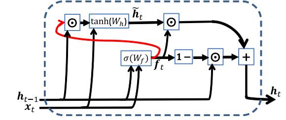
Let’s take a look at the structure of the minimal GRU:


Source: Minimal Gated Unit for Recurrent Neural Networks
The first equation f is the forget gate, the second equation, if you compare it with the previous RNN, you will find it has the same structure, only that the forget gate f controls how much previous information each neuron lets out (changing the states of other neurons), and the third equation describes “inertia”, that is, how much previous value each neuron maintains and how much it updates.
If you understand this structure, you understand the essence of memory RNN.
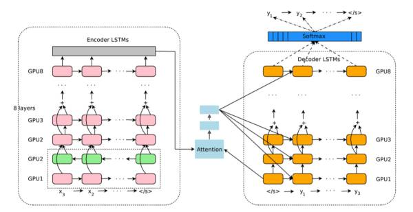
Now it’s time to see how Google Translate works. First, translation is about communicating between two different languages, and the essence of this communication is that the concepts they express are the same. When our brain translates, it also relies on the concepts being the same, such as apple-vs-苹果, to communicate between the two languages. If Chinese is the input and English is the output, what the neural network actually does is:
Encoding: Using an LSTM to convert Chinese into neural code
Decoding: Using another LSTM to convert neural code into English.
The output of the first LSTM becomes the input of the second LSTM, and the two networks can be trained with a large corpus. The groundbreaking method that Google introduced in 2016 incorporated an attention mechanism, making Google’s translation system closer to human brain functionality.

The core advantage of using memory neural networks for translation is that we can flexibly combine contexts, achieving transitions from sentence to sentence and paragraph to paragraph, because the memory characteristics allow the network to integrate information across different time scales rather than just focusing on individual words. This is akin to grasping the context rather than just taking words at face value. It is also because of this that RNN has endless imaginative applications, and we will continue to discuss Google Translate and various applications of RNN in the next article.
References:
The Unreasonable Effectiveness of RNN Google’s Neural Machine Translation System: Bridging the Gap between Human and Machine Translation
Minimal Gated Unit for Recurrent Neural Networks
More Reading
What AlphaGo’s Victory Tells Us
A Feast of Interdisciplinary Neural Networks
Support Vector Machines in the Brain
