
Machine learning is essentially a search in space and generalization of functions. Now enterprises mainly rely on supervised learning based on samples. In reality, logistic regression (LogisticRegression, LR) has a fast training speed and strong interpretability, but its fitting accuracy is insufficient. On the other hand, support vector machines (SupportVectorMachine, SVM) have high prediction accuracy, but feature selection and parameter tuning are very difficult. Often, one cannot have both. Due to its advantages such as automatic feature selection, low computational complexity, and good generalization effect, the XGBoost algorithm has been adopted by many data mining experts.
Today, let’s explore the XGBoost algorithm again to clarify what XGBoost is all about. XGBoost is an optimized algorithm based on boosting algorithms like AdaBoost and GBDT. Generally speaking, an algorithm consists of three parts: the model, parameters, and objective function. The model can be understood as a combination of basis functions (fixed forms of a function, meaning the function will only change based on this function and will not lose its essence) and weights, which together form an algorithm for a certain type of problem. Parameters are the results of the algorithm’s learning, just like the paths q from the root node to the leaf nodes produced by decision tree learning and the expected weights w at each leaf node. Changing the parameters (q, w) means altering the existing model. The optimization of the objective function needs to achieve two goals: first, to make the predicted values as close as possible to the actual values; second, to ensure the model’s generalization ability (GeneralizationAbility). To achieve the first goal, we can minimize the loss function, and for the second goal, we can add a penalty term that controls the model’s complexity during the minimization of the loss function, which can also be referred to as regularization terms, such as L1 and L2 losses. We optimize the objective function to achieve an optimal balance between error and complexity.
Given the objective functionObj:
Obj(x) = L(x) + O(x)
The objective functionObj(x) consists of two parts: the error function L(x) and the complexity function O(x). Our learning goal is certainly to minimize the loss bias and keep the function as simple as possible. High complexity implies a high risk of overfitting. Ultimately, we are concerned with the size of the generalization error (TotalError), which is the balance point between bias (Bias) and variance (Variance). Bias measures the deviation of the expected prediction of the learning algorithm from the actual result, reflecting the fitting ability of the learning algorithm itself; variance measures the change in learning performance caused by variations in the training set of the same size, reflecting the impact of data perturbations.
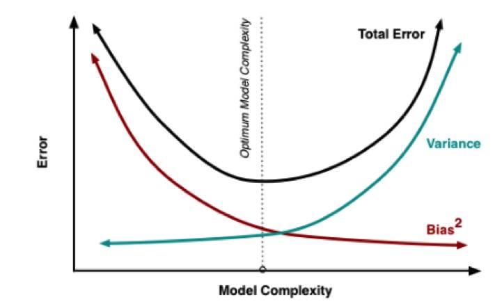
From the above figure, we can see that the minimum point of the generalization error (TotalError) is the optimal point of the model, indicating that the model’s generalization ability is the best. Before the minimum point of the generalization error, we call the model underfitting (Underfit); after the minimum point of the generalization error, we call the model overfitting (Overfit).
Next, let’s see how XGBoost is specifically implemented. First, we have our base learner. The base learner can choose weak classifiers (WeakClassifier) like decision trees or logistic regression as the foundation classifier. The idea of XGBoost is to learn the loss value after learning in each iteration, adding the predicted values of the base classifier to predict the results. The weaker the classifier, the larger the bias, because each learning step reduces bias, and more models will participate in judgment. In fact, setting a smaller learning rate (Shrinkage) results in a larger number of models. The underlying idea of the boosting algorithm is similar to: weak classifiers are like students who are only good at certain subjects; during the learning process, the classifier will choose the best students in that subject, and in the end, a group of specialized students will complete an exam together.
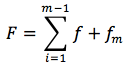
Weak classifiers can only achieve good classification through combination, which is different from the traditional SGD (Stochastic Gradient Descent) algorithm. The traditional SGD algorithm seeks a functionf that minimizes the squared loss function in the training set. We refer to predicting results through the stacking of weak classifiers as an additive model.
The fitting of the additive model is achieved through an iterative process (backward fitting algorithm) that smooths each predictor variable. The algorithm must balance fitting error and degrees of freedom to ultimately achieve optimality.
We choose the basis function regression tree (RegressionTree), also known as CART tree, which is the decision tree for regression problems. The choice of CART tree is based on prior knowledge.
CART can often also act as a strong classifier, as long as the depth of the tree is sufficient, it can classify samples well, but it has overfitting issues. Therefore, when learning the XGBoost model using CART, we must control the tree depth because we need weak classifiers. Random forests are an ensemble of decision trees implemented from the perspective of SGD and BootStrap and solve most of the sample feature selection and overfitting problems. In fact, XGBoost implements a more powerful classifier from the perspective of the additive model.
Choosing the basis function CART, we assume the m-th prediction result of CART
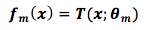
The basis function determines our loss function, and the functionT represents the decision tree, m represents the number of decision trees or weak classifiers, theta represents the area division of the decision tree (which can be understood as: the partition path of the decision tree) and the constants of each area. Our final prediction result isf(m-1)+T(m), wheref(m-1) is the accumulated result of the previous m-1 predictions, and the final error term is
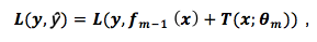
L is the sum of the differences between the true values and the predicted values. Thus, our error loss has been quantified.
CART classifies by optimizing the GINI index, pruning, and controlling tree depth. The underlying principle is similar to controlling the complexity of the model and the maximum likelihood estimation of regularization. The complex function we designOmega is actually based on this idea. The number of leaf nodesT and the square of the L2 norm of LeafScore define the structural complexityOmega function:
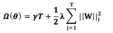
In the above formula: γ (gamma) is the threshold, the coefficient of the number of leaf nodes T, similar to XGBoost’s pre-pruning, and the coefficientλ (lambda) is the coefficient of the square of the L2 norm of LeafScore in the regularization term, which smooths LeafScore and also helps prevent overfitting.
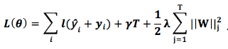
The combined error function and complexity function can be expressed as follows:
Next is the key point:
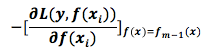
The traditional GBDT algorithm (without considering the penalty termOmega) calculates the loss function in each iteration to maximize the reduction of its error, which is what we call the gradient descent algorithm. As long as we follow the negative gradient direction, we can ensure maximum reduction in each iteration, thus optimizing the algorithm. By summing the weak classifiers from each iteration, we can make our additive model (GeneralizedAdditiveModels) results as optimal as possible.
After deriving the loss function, the area divisions and constants of each CART are known, so each CART can be determined.
However, the gradient algorithm is just an abstraction, and there will be many weak classifiers. So we must provide a general algorithm:
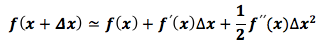
Taylor expansion is a more general approximation algorithm and can be implemented directly in source code.
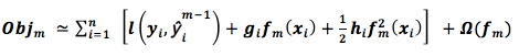
The objective function:
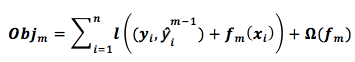
n represents the number of samples, m represents the iteration number,f(m) represents the error of the m-th iteration.
Using Taylor expansion:
Definition:
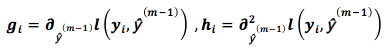
Substituting for calculation:
This objective function has a very obvious characteristic; it only depends on the first and second derivatives of the error function for each sample point.
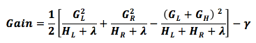
You must be confused and wonder what these formulas are for. In fact, it is very simple; the goal is to find the optimal feature split point with the lowest complexity, similar to the GBDT idea without complexity. The classification metrics of the base learner can also be likened to CART trees, which increase the complexity of the Gini index GiniIndex. After arranging the features, we can traverse each dimension of the feature and evaluate each split point’sGain value to determine the optimal split point.
Thus, the source of the formulas and the learning principles of XGBoost have been explained.
Characteristics of XGBoost:
1. XGBoost algorithm can be used for linear classification and can be viewed as a linear regression algorithm with L1 and L2 regularization.
2. XGBoost uses second-order Taylor expansion similar to Newton’s method during computation, so it requires the objective function to be continuously differentiable up to the first and second order.
3. Compared to traditional GBDT, it has added regularization functions, thus significantly improving the prevention of overfitting.
4. In terms of distributed algorithms, XGBoost sorts each dimension of features within a single machine and saves them in a Block structure. Thus, multiple feature calculations can be executed across different machines, and the results are aggregated at the end. This gives XGBoost the ability for distributed computation.
5. Since feature values are only used for sorting, outlier feature values have little impact on the learning of the XGBoost model.
6. Each calculation only selects the feature with the maximum gradient reduction, so the issue of feature correlation selection is also resolved.
7. XGBoost includes complexity functions, and the entire splitting method is the same.