All econometrics methodologiesCode programsMacro and microdatabases and various softwareare all shared in the community. Welcome to exchange and visit the econometrics circle community.
Regarding machine learning methods, refer to the following articles:1Machine learning methods have appeared in top journals such as AER, JPE, QJE!, 2Frontier: A summary of the applications of machine learning in finance and energy economics, 3What are the steps, tools, methods, and visualizations for text analysis?4 A comprehensive literature review on the application of big data text analysis in economics and finance,5The most comprehensive: A summary and outlook on the application of deep learning in economic and financial management, which young and middle-aged scholars cannot ignore!6Top Frontier: Machine learning in agriculture and applied economics, and its comparison with econometrics, if you don’t read it, you’ll be out!7Machine learning and big data econometrics, you must read this article, 8Book recommendations on machine learning and econometrics, classics worth having, 9The latest trends in the application of machine learning in microeconometrics: big data and causal inference,10The first book on machine learning, data mining, reasoning, and prediction, 11Top, machine learning is an applied econometric method, not understanding it will face the risk of elimination in the future!12The latest: Research on the impact of Wuhan’s lockdown on air pollution and health using machine learning and synthetic control methods!13Chen Shuo: A review and outlook on machine learning in economic research,14Research progress on the impact of machine learning on economic research
Main TextAuthor: Wang Biaoyue, School of Software and Microelectronics, Peking University; Contact Email:[email protected]KNN, known as K-Nearest Neighbor in Chinese, is used to select k nearest samples for a given sample point. As an introductory algorithm in machine learning, the NN in KNN, although it shares a literal meaning with the NN matching in the PSM model of econometrics, has essential differences in algorithm principles.PSM: The NN matching is based on the probability or score of the sample entering the “treatment group” (propensity score), usually calculated using logit/Probit functions. Two observed values are considered close if their probabilities or scores are similar.KNN: The proximity of neighbors is measured by distance. In Stata and R (using the knn3 function), the default distance is the Euclidean distance (Euclidean Distance, denoted as L2).In recent years, econometrics has also incorporated KNN as a non-parametric estimation method. KNN can be seen as an instance-based learning algorithm that approximates locally and defers all calculations until after classification, hence it is also called an “lazy learning algorithm.” KNN classification infers the category of the target sample based on the categories of the k nearest neighbor samples.
1 KNN Algorithm Principles
KNN is a common algorithm in machine learning, applicable to both classification and regression.
1.1 Classification Algorithm Principle
Definition of Euclidean distance:Here x and y represent two sample observation vectors, indicating the specific value of the i-th feature variable of sample x, indicating the specific value of the i-th feature variable of sample y.KNN classification algorithm principle: The classification result of an object is determined by its k nearest neighbors (usually between 1 and 5), also known as “vote.” That is, among the k nearest neighbors, the category with the highest frequency is considered the category of the object under consideration. For example, when discussing whether a student is a top student or a poor student (only two classifications), we observe the k closest friends, and if the proportion of top students is the highest, we classify this student as a top student, otherwise as a poor student. This is somewhat similar to the common saying “birds of a feather flock together” — the properties of the nearest k samples determine the properties of the target sample.
1.2 Regression Algorithm Principle
In KNN regression, the output is the average value of the result variable of the k nearest neighbor samples of the target object. For example, the income level of an individual equals the average income levels of their k closest friends. Due to space limitations, this article does not provide detailed case studies on KNN regression.
1.3 General Steps of the KNN Algorithm
(1) Determine the value of k, preferably an odd number (an even number may lead to ties); choose the algorithm for measuring neighbor distance, the default is L2 Euclidean distance.(2) Split the original data into a training dataset (e.g., 70%) and a testing dataset (e.g., 30%).(3) Build a learning algorithm model based on the training dataset.(4) Make predictions based on the testing data to evaluate the performance of the learning algorithm model.(5) Repeat steps (3) and (4) to select the optimal model.
1.4 Advantages of the KNN Algorithm
(1) Simple yet powerful. The logic is straightforward, no parameter estimation is required; easy to understand and implement.(2) Versatile. It can handle binary and multi-class problems, as well as regression problems. In multi-class predictions, it typically performs better than another common machine learning algorithm, SVM (Support Vector Machine).(3) Compared to algorithms like Naive Bayes, it is less sensitive to outlier sample points.
1.5 Limitations of the KNN Algorithm
Firstly, the KNN algorithm is very sensitive to the local structure of the dataset and the value of k. For instance, in the example of classifying top students, if k=1 and the target student is a top student, then the target student is classified as a top student; if k=3, and among the neighbors, 2 are poor students and 1 is a top student, then the target student is classified as a poor student; if k=5, with 2 poor students and 3 top students, the target student again becomes a poor student. This simple example shows that changes in the model parameter k directly affect the classification results.Secondly, when k is small, the instances used for training come from a small neighborhood, reducing the approximation error but increasing the prediction error. This means the smaller k is, the more complex the model becomes, and it is more likely to overfit (overfitting refers to a model that performs well on training data but poorly on unseen data). When k is large, the instances used for training come from a larger neighborhood, reducing estimation error but increasing approximation error. The larger k is, the simpler the model becomes. In extreme cases, considering k=N sample observations, the classification algorithm results will all become the largest category in the dataset, and the regression algorithm results will all become the mean of the dataset.Thirdly, when classifying or predicting new data, KNN must search for the nearest old samples through testing data for judgment. Therefore, when the dataset is large, the KNN algorithm in Stata or R can consume a lot of memory and lead to slow execution. In cases of high dimensionality, the “curse of dimensionality” problem may also arise.Lastly, as a lazy machine learning algorithm, KNN is quite lazy and hardly learns.
2 Implementation of KNN in Stata and R
2.1 Implementation of KNN in Stata
The command to implement KNN classification in Stata is “discrim knn.” Unfortunately, as of Stata 16, the official version and SSC have not provided a regression command based on KNN. The “discrim knn” command can also calculate similarity and dissimilarity using various specific algorithms.Syntax: discrim knn varlist [if] [in] [weight], group(groupvar) k(#) [options]Explanation: Here varlist refers to the list of (feature) variables; groupvar refers to the grouping variable or label variable, i.e., the result variable or dependent variable in econometrics. In machine learning, different categories of samples are labeled with different labels to indicate classification.Common options include the following:(1) k(#), where # represents the number of KNN, defaulting to k=1.(2) priors, which refer to the prior probabilities of the groups, defaulting to equal probabilities. Another common option is proportional, which uses the grouping frequency/total sample size as the corresponding probability.(3) measure, defaulting to L2, Euclidean distance.(4) notable and lootable, used to report compressed replacement classification result tables and report leave-one-out classification result tables, respectively.(5) ties, which handles situations where the classification results of the k nearest neighbor samples are equal and cannot be determined, including marking as missing values and random selection, etc. In practical operations, we can consider using an odd k, which generally avoids the ties problem.
2.2 Implementation of KNN in R
Common functions for implementing the KNN algorithm in R include three: (1) the knn3 function in the caret package; (2) the knn function in the class package; (3) the kknn function in the kknn package. This article uses the knn3 function; specific implementation steps are found in section 3.2.
3 Case Study: Classification and Prediction of Neighborhood Types
The goal of this case study is to predict the type of a neighborhood (wealthy area or ordinary area) based on several feature variables of a neighborhood.Here is a brief introduction to the data used in this case study, “houseprice_10000.csv.” This data is adapted from real housing price data from a certain state in the United States: N=10000; using community neighborhoods as the basic unit; other variables characterize the neighborhood from aspects such as per capita income. A new variable, rich, has been generated based on the original data. The names, meanings, and values of all variables are shown in the table below.
Variable Name
Variable Type
Meaning and Values
communityid
Feature Variable
Neighborhood coding id, from 1 to 10000. Not included in the model
income
Feature Variable
Per capita income level of the neighborhood, in dollars
houseage
Feature Variable
Average age of houses in the neighborhood, in years
rooms
Feature Variable
Average number of rooms in houses in the neighborhood, in units
population
Feature Variable
Total population of the neighborhood, in units
houseprice
Result Variable – Continuous
Average price of houses in the neighborhood, in dollars
rich
Result Variable – Categorical
Generated based on houseprice, greater than the overall sample mean takes 1 (wealthy area), otherwise takes 0 (ordinary area)
3.1 Stata Modeling and Prediction
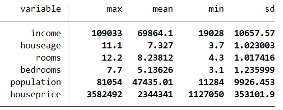
The specific process of implementation in Stata is as follows (complete code can be found in the do file). First, organize the data into a format suitable for Stata modeling.. cd “D:\R” // Change working directory . import delimited “D:\R\houseprice_10000.csv”, clear // Import original data * View summary statistics of key variables . tabstat income-houseprice, stat(max mean min sd) column(statistics)
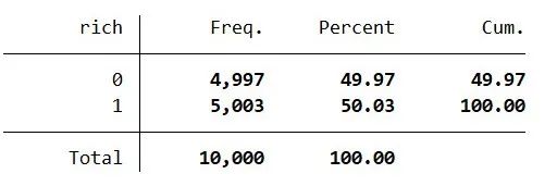
. gen rich = 1 if houseprice >= 2344341 // Generate wealthy area rich variable(4,997 missing values generated). replace rich = 0 if mi(rich)(4,997 real changes made). tab rich
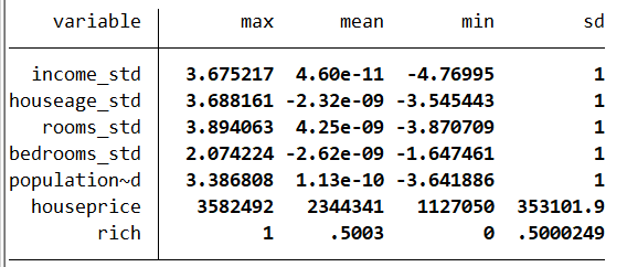
. label define rich_lb 0 “Ordinary Area” 1 “Wealthy Area”. label values rich rich_lb. set seed 1898. gen rand=runiform() // Generate random numbers to ensure random sampling for model training. sort rand. **Standardize several key feature variables to eliminate the influence of units (dimensions). foreach var of varlist income – population {2. egen var'_std = std(var’)3. }**View the general situation of standardized data. tabstat income_std-population_std houseprice rich, ///stat(max mean min sd) column(statistics)
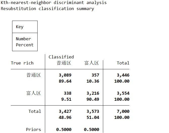
Second, randomly sample 7000 out of 10000 original samples as the training dataset to build the KNN model.* Stata KNN classification model modeling based on the first 7000 samples. The number of neighbors k is set to 15 . discrim knn income_std-population_std in 1/7000, k(15) group(rich). dis (3089+3216)/7000 // The prediction accuracy of the training data itself is 0.9007
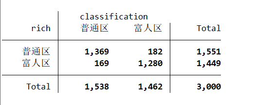
Third, based on the remaining 3000 testing datasets, predict whether the neighborhood is a wealthy area or an ordinary area.. predict rich_hat in 7001/10000, classification // Predict based on 3000 testing data(7000 missing values generated). label values rich_hat rich_lb. tab rich rich_hat in 7001/10000
Fourth, compare the model prediction results with the actual testing data to evaluate the accuracy of the predictions.. dis (1369+1280)/3000 // The prediction accuracy of the training data itself is 0.883.885Due to the high similarity of the data itself, k is set to 15 in this case, and the final prediction accuracy is 0.883. After further attempts, it was found that when k is approximately 129, the accuracy reaches 0.887; thereafter, as k increases, the accuracy starts to decline. It can be estimated that the optimal model’s k is around 129.
3.2 R Modeling and Prediction
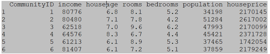
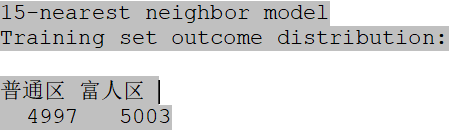
The modeling process of the KNN classification algorithm in R is similar to that in Stata, but the specific operations differ significantly.First, organize the data into a format suitable for R modeling.#Using KNN to classify wealthy and ordinary areas###########################################Load related packageslibrary(caret)library(e1071) set.seed(1898) # Before setting the seed, the original data may need to be sorted to ensure repeatability of results####Prepare original datarm(list=ls()) # Clear all data in the current working environmenthouse <- read.delim(“D:/R/houseprice_10000.csv”, sep=”,”) # Import data summary(house$houseprice) # View the general situation of the housing price scalar
head(house) # View the head of the data
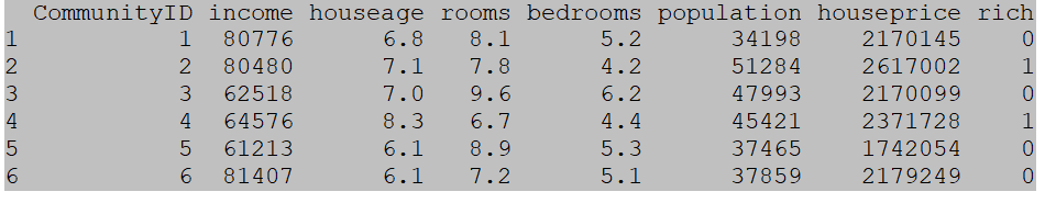
house$rich <- ifelse(house$houseprice >= mean(house$houseprice), 1, 0) # Define neighborhoods with above-average prices as “wealthy areas”, otherwise as “ordinary areas”head(house)
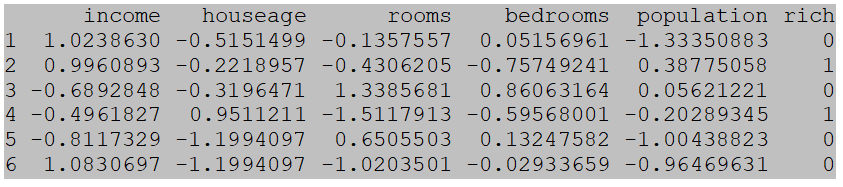
house <- house[-c(1,7)] # Remove useless variables communityid and housepricehouse[1:5] <- apply(house[1:5], 2, scale) # Standardize variables except for the result variablehead(house)
Second, randomly sample 7000 from the 10000 original data to create the training dataset, while the remaining 3000 samples form the testing dataset.####Prepare training and testing datahouse$rich <- factor(house$rich, # Key step! Convert rich variable to factor variable+ levels=c(0,1),+ labels=c(“Ordinary Area”, “Wealthy Area”))labels <- house$rich # Save rich variable into labels vector# Use the createDataPartition function in the caret package to perform random sampling and splitting of data index <- createDataPartition(house$rich, p=0.7) # 70% for training datatrain_house <- house[index$Resample1, ] # Extract training data from the total sample train_lab <- labels[index$Resample1] # Extract classification labels for training data test_house <- house[-index$Resample1, ] # The remaining data is for testingtest_lab <- labels[-index$Resample1] # Extract classification labels for testing data# View(train_lab) # View classification labels for training data# View(test_lab) # View classification labels for testing dataThird, based on the remaining 3000 testing datasets, predict the type of the neighborhood (wealthy area or ordinary area)####KNN Modelinghouse_m1 <- knn3(rich~., house, k=15) # rich is the result variable, others are feature variableshouse_m1
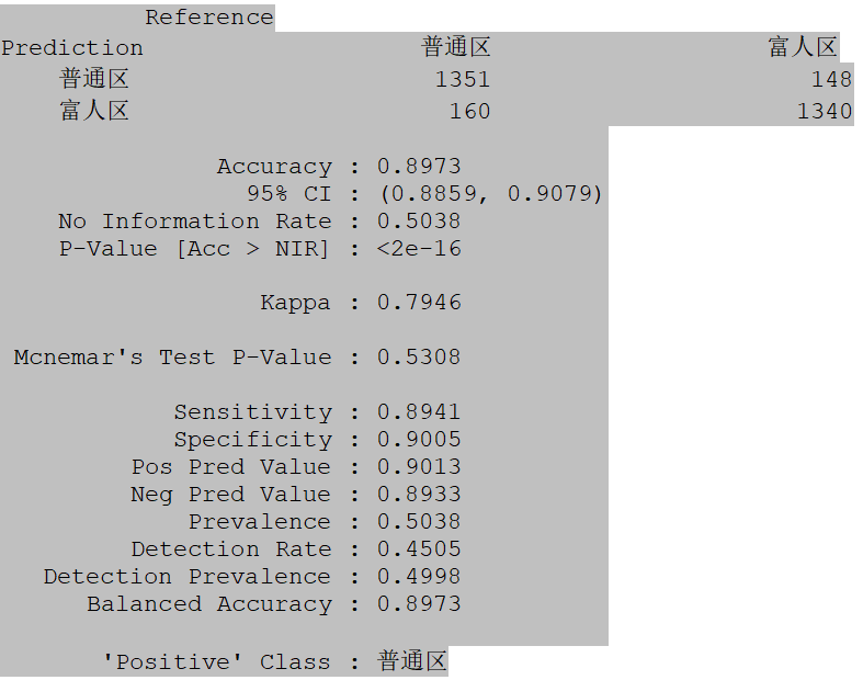
Fourth, compare the model prediction results with the actual testing data to evaluate the accuracy of the predictions.rich_hat <- predict(house_m1, test_house, type=”class”)test_lab <- as.factor(test_lab)rich_hat <- as.factor(rich_hat)confusionMatrix(test_lab, rich_hat) # Use confusion matrix function to display testing results
The results of the confusion matrix show that the model (k=15) has a prediction accuracy of 0.8973, which is close to the Stata model (k=15) of 0.883. Regardless of whether in Stata or R, the overall prediction accuracy of neighborhood types is not very high, but still acceptable. The reason for the larger k in this case is that part of the data is adapted from real existing data, leading to high similarity, thus a larger k value is used.
3.3 Comparison of Stata and R Modeling
(1) Implementation Efficiency: Overall, Stata operations are simpler. As a commercial software, Stata indeed provides users with an extremely convenient and efficient experience. However, the steps in R, while more numerous, are very rigorous and clear. It should be noted that compared to Stata’s command-based modeling, R is true “programming,” which is why learning and using R and Python can indeed make one’s thinking clearer and more rigorous.(2) Comparison of Modeling Methods: In this regard, Stata cannot compare with R at all. As of the 2019 version 16, Stata still does not provide a command for KNN regression algorithms, while R already has multiple functions for KNN classification and regression (knn, kknn, knn3, and knnreg). R also provides functions for finding the optimal model, making it easier for users to quickly identify the best k value; interested readers can further study this.(3) Post-Modeling Analysis: In this regard, Stata is clearly superior, as KNN modeling in Stata provides a series of commands for post-estimation, allowing for a more detailed presentation of the learning algorithm model.Summary: R and Stata each have their strengths and weaknesses. The differences in their styles are mainly because R represents the mainstream trend in machine learning, with algorithms and terminology closer to Python, while Stata emphasizes introducing KNN and other machine learning models from the perspective of economics and econometrics.
4. Conclusion
Since the perspectives of R or Python in introducing machine learning algorithms differ significantly from econometrics, is it still necessary to spend a lot of time learning them? Considering that Python has now grown to be the world’s leading programming language and R is the world’s leading statistical language, both being open-source software, their replacement (or partial replacement) of traditional commercial statistical software is an inevitable trend. Only by familiarizing and mastering the two most mainstream languages for machine learning, Python or R, can we keep pace with the era of artificial intelligence.As for the comparison between R and Python, personally, I recommend R. After all, Python is a general-purpose programming language, with thinking and logical perspectives leaning more towards computer science, while R is inherently a statistical language, more closely related to econometrics, making it more suitable for friends in management and economics disciplines.In summary, the combination of R and Stata can help us master mainstream machine learning algorithms while allowing us to better grasp machine learning from an econometric perspective, enabling the use of machine learning for causal inference in future economic research.PS: Regarding the introduction of KNN for regression modeling and prediction in R, I have completed the first draft and will send it out as soon as possible. Welcome everyone to follow this public account for subsequent KNN-related articles.
5. References
(1) Chen Qiang, “Advanced Econometrics and Stata Applications,” Second Edition.(2) Xue Zhen, Sun Yulin, “Statistical Analysis and Machine Learning in R Language”.(3) Athey S, Imbens G W. Machine Learning Methods Economists Should Know About[J]. Research Papers, 2019.(4) Athey S. The Impact of Machine Learning on Economics[J]. Nber Chapters, 2018.(5) A large number of official help files related to the KNN algorithm in Stata and R.Attached Data and Code:Link to Attached Data and Code:https://pan.baidu.com/s/1nvnQdrky83H8GTeP9NHQtwExtraction Code:jlsq
For related econometric methods video courses, articles, data, and code, refer to 1. Free course on panel data methods, articles, data, and code all here, excellent scholars should collect and study!2. Free course on difference-in-differences (DID) methods, articles, data, and code all here, excellent scholars must collect and study!3. Free course on instrumental variable (IV) estimation, articles, data, and code all here, don’t regret not studying!4. Free course on various matching methods, articles, data, and code all here, mastering matching methods is not a dream!5. Free course on regression discontinuity (RD) and synthetic control methods (SCM), articles, data, and code all here, necessary to study seriously!6. Free course on spatial econometrics, articles, data, and code all here, spatially related scholars please pay attention!7. Free video courses on Stata, R, and Python, articles, data, and code all here, really useful!
The following short link articles belong to a collection, which can be saved for reading, otherwise, it will be difficult to find later.
2.5 years, nearly 1000 non-repetitive econometric articles in the Econometrics Circle,
You can directly search for any econometric-related questions in the public account menu,
Econometrics Circle
Data Series:Spatial Matrix | Industrial EnterpriseData | PM2.5 | Marketization Index | CO2 Data | Nighttime Lights| Official Dialects | Micro Data| Internal DataEconometric Series:Matching Methods | Endogeneity | Instrumental Variables | DID | Panel Data | Common Tools | Moderation and Mediation | Time Series | RDD Discontinuity | Synthetic Control | 200 Articles Collection | Causal Identification | Social Networks | Spatial DIDData Processing:Stata | R | Python | Missing Values | CHIP/ CHNS/CHARLS/CFPS/CGSS, etc. |Useful Series:Energy and Environment | Efficiency Research | Spatial Econometrics | International Trade | Econometric Software | Business Research | Machine Learning | SSCI | CSSCI | SSCI Query | Expert ExperienceThe Econometrics Circle has organized an econometric community with the following characteristics:Most enthusiastic and helpful,Most cutting-edge trends,Most social science materials,Most social science data,Most research experts,Most overseas prestigious universities. Therefore, it is recommended that actively ambitious and passionate young and middle-aged scholars engage in discussions and exchanges within the community, always believing that excellence is achieved through mutual influence and support.