I previously wrote two articles on address processing, detailed below:
Address Processing in Risk Control: Simple and Effective Regex Replacement
Address Processing in Risk Control: Simple, Accurate, and Effective Multi-label Clustering
Today we are writing the third article, using KNN to construct similar addresses. Although this article is about addresses, many scenarios can draw on this, so everyone should learn to think outside the box.
Additionally, many students do not master algorithms deeply enough; they might find a demo and run a case, thinking they are very skilled. However, many of our algorithms are quite profound. If you don’t understand today’s article, you can review my previous articles:KNN Algorithm Simple? I Spent 30,000 Words Not Making It Clear…
If you want to learn more deeply and systematically, you can also buy my course, which explains a similar case in great detail.
Let’s start with the main content. First, let’s look at the format of the address data. The previous articles also used this dataset. To practice with the data, please follow Little Wu Talks Risk Control and reply with 【Address Data】 to get the download link.
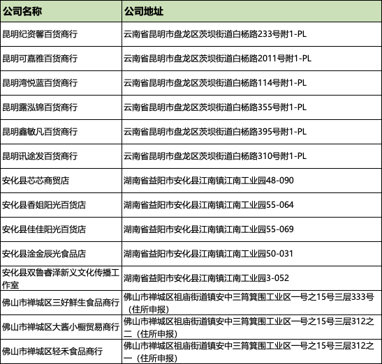
Today we won’t do regex processing, let’s get straight to it.
# Load the necessary packages
import pandas as pd
import numpy as np
import os

# Read data - For data, please follow "Little Wu Talks Risk Control" and reply with 【Address Data】
os.chdir('/Users/wuzhengxiang/Documents/DataSets/Address Processing')
data = pd.read_csv('Company Address Data.csv')
print(data.head(20))

# Jieba word segmentation - test
import jieba
jieba.lcut('Little Wu is the most handsome in the universe')  # ['Little Wu', 'is', 'the', 'most', 'handsome', 'in', 'the', 'universe']

# Perform word segmentation with Jieba

df = data
df = df['Company Address'].apply(lambda x: ' '.join(jieba.lcut(x)))
df.head()

# Vector transformation
tf-idf_vectorizer_word = TfidfVectorizer(max_features=20000,
                             token_pattern=r"(?u)\b\w+\b",
                             min_df=1,
                             analyzer='word',
                             ngram_range=(1, 2)
                             )
vectorizer_word = tf-idf_vectorizer_word.fit(df)
tfidf_matrix = vectorizer_word.transform(df)
# Check the size of the vocabulary
print(len(vectorizer_word.vocabulary_))  # 109
# Check some words in the vocabulary
vectorizer_word.vocabulary_{'Yunnan Province': 51, 'Kunming City': 72, 'Panlong District': 85, 'Ciba': 93, 'Street': 95, 'Baiyang': 81, 'Road': 98, '233': 13}
With the above code, we obtained the vector representation of the text. Next is the KNN algorithm.
The radius_neighbors_graph constructs a restricted radius neighbor graph, meaning neighbors within a certain distance are included, while those beyond that distance are excluded. We can also use kneighbors_graph to find the same number of neighbors for each node.
from sklearn.neighbors import radius_neighbors_graph
from sklearn.neighbors import kneighbors_graph

# Construct the restricted radius neighbor graph. We can also use kneighbors_graph to find the same number of neighbors for each node.
A = radius_neighbors_graph(tfidf_matrix,
                      radius=0.99,
                      mode='connectivity',
                      include_self=False
                           )
A.toarray()
array([[0., 1., 1., 1., 1., 1., 0., 0., 0., 0., 0., 0., 0., 0.],
       [1., 0., 1., 1., 1., 1., 0., 0., 0., 0., 0., 0., 0., 0.],
       [1., 1., 0., 1., 1., 1., 0., 0., 0., 0., 0., 0., 0., 0.],
       [1., 1., 1., 0., 1., 1., 0., 0., 0., 0., 0., 0., 0., 0.],
       [1., 1., 1., 1., 0., 1., 0., 0., 0., 0., 0., 0., 0., 0.],
       [1., 1., 1., 1., 1., 0., 0., 0., 0., 0., 0., 0., 0., 0.],
       [0., 0., 0., 0., 0., 0., 0., 1., 1., 1., 1., 0., 0., 0.],
       [0., 0., 0., 0., 0., 0., 1., 0., 1., 1., 1., 0., 0., 0.],
       [0., 0., 0., 0., 0., 0., 1., 1., 0., 1., 1., 0., 0., 0.],
       [0., 0., 0., 0., 0., 0., 1., 1., 1., 0., 1., 0., 0., 0.],
       [0., 0., 0., 0., 0., 0., 1., 1., 1., 1., 0., 0., 0., 0.],
       [0., 0., 0., 0., 0., 0., 0., 0., 0., 0., 0., 0., 1., 1.],
       [0., 0., 0., 0., 0., 0., 0., 0., 0., 0., 0., 1., 0., 1.],
       [0., 0., 0., 0., 0., 0., 0., 0., 0., 0., 0., 1., 1., 0.]])
Next, we will use the maximal connected subgraph to mine:
import networkx as nx
import matplotlib.pyplot as plt

# Convert data into graph format
G = nx.from_numpy_matrix(A.toarray())

# Find all connected subgraphs
com = list(nx.connected_components(G))

# Organize the list-dictionary into a tabular format
df_com = pd.DataFrame()
for i in range(0, len(com)):
    d = pd.DataFrame({'group_id': [i] * len(com[i]), 'user_id': list(com[i])})
    df_com = pd.concat([df_com, d])

# View the results
df_com   group_id  user_id
0         0        0
1         0        1
2         0        2
3         0        3
4         0        4
5         0        5
6         1        0
7         1        1
8         1        2
9         1        3
10        1        4
100        2       11
111        2       12
122        2       13
We have obtained the group divisions of each sample. To make it more intuitive, we will visualize the next step, which is relatively complex, so please study it carefully.
# Restore the group clustering data back to the original data
data['group_id'] = pd.Series(group_id)
pd.Series(group_id).value_counts().head(20)
# View a specific group
data[data['group_id'] == 0].sort_values(by='Company Name')
Company Name Company Address group_id
1 Kunming Kejiaya Department Store Yunnan Province Kunming City Panlong District Ciba Street Baiyang Road 2011 No. 1-PL 0
2 Kunming Wanyuelan Department Store Yunnan Province Kunming City Panlong District Ciba Street Baiyang Road 114 No. 1-PL 0
3 Kunming Jizixin Department Store Yunnan Province Kunming City Panlong District Ciba Street Baiyang Road 233 No. 1-PL 0
4 Kunming Xuntufa Department Store Yunnan Province Kunming City Panlong District Ciba Street Baiyang Road 310 No. 1-PL 0
5 Kunming Xinminfan Department Store Yunnan Province Kunming City Panlong District Ciba Street Baiyang Road 395 No. 1-PL 0
6 Kunming Luhongjin Department Store Yunnan Province Kunming City Panlong District Ciba Street Baiyang Road 355 No. 1-PL 0
# Extract the text of the visualized group
comment_group = data['Company Address'][data[data['group_id'] == 0].index].reset_index(drop=True)
labels = dict(comment_group)
labels
# Extract the tf-idf of the visualized group
tfidf_group = tfidf_matrix.toarray()[data[data['group_id'] == 0].index]
# Recalculate the connectivity matrix
A = radius_neighbors_graph(
tfidf_group,
radius=0.99,
mode='connectivity',
include_self=False
)
# Visualize the address data
import networkx as nx
import matplotlib.pyplot as plt
# Convert matrix format to graph format
G = nx.from_numpy_matrix(A.toarray())
## Solve the issue of displaying Chinese characters in the graph
plt.rcParams['font.sans-serif'] = ['Arial Unicode MS']
plt.rcParams['axes.unicode_minus'] = False
# Color settings
colors = ['r', 'c', 'y', 'c'] * 1000
#colors = ['#008B8B', 'r', 'b', 'orange', 'y', 'c', 'DeepPink', '#838B8B', 'purple', 'olive', '#A0CBE2', '#4EEE94'] * 500
colors = colors[0:len(G.nodes())]
#kamada_kawai_layout spring_layout
plt.figure(figsize=(4, 4), dpi=400)
nx.draw_networkx(G,
pos=nx.spring_layout(G),
node_color=colors,
labels=labels,
node_size=500,
font_size=5,
width=0.2,
alpha=1)
plt.axis('off')
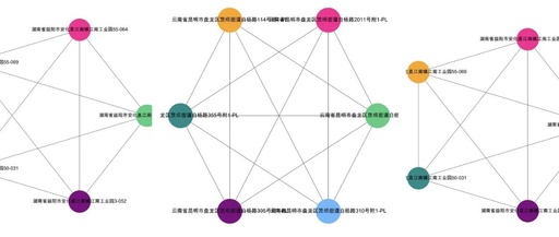
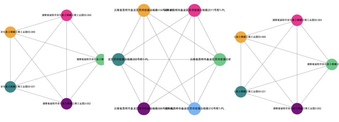
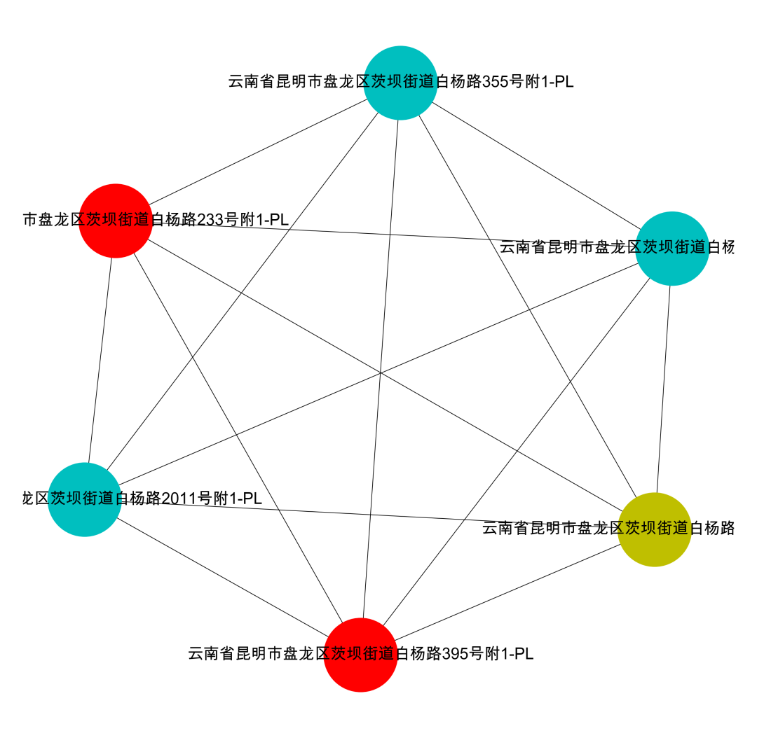
plt.show()Visualization Result: data[‘group_id’] == 0
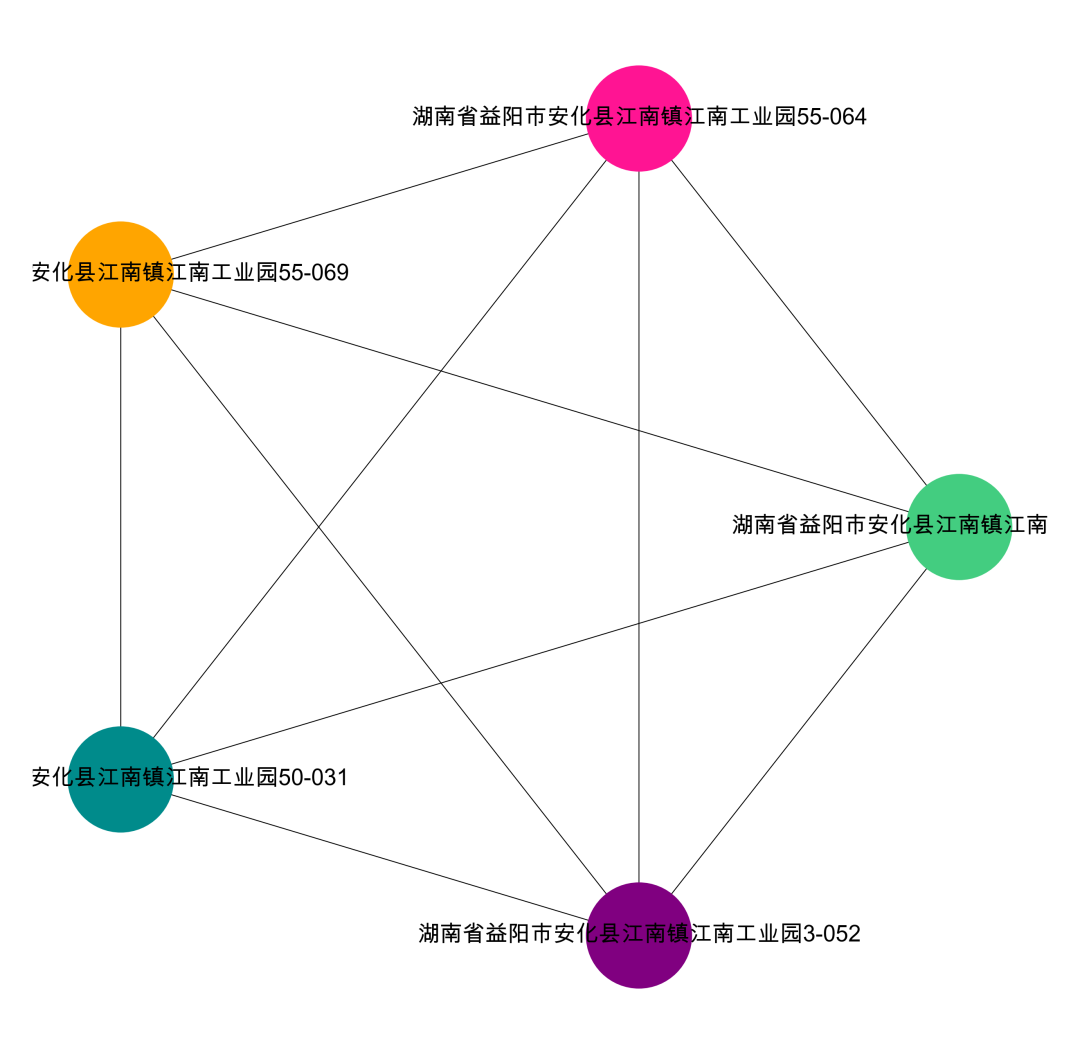
We can look at the visualization of other groups.
Visualization Result: data[‘group_id’] == 1
Visualization Result: data[‘group_id’] == 2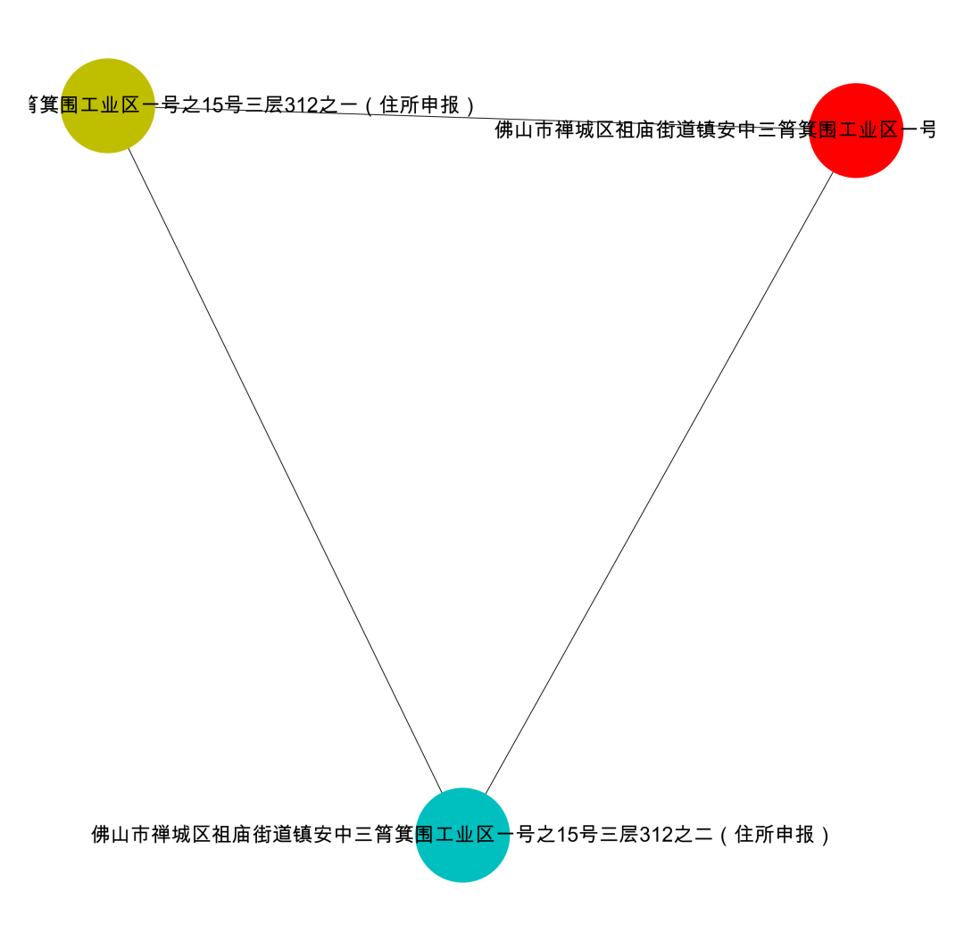
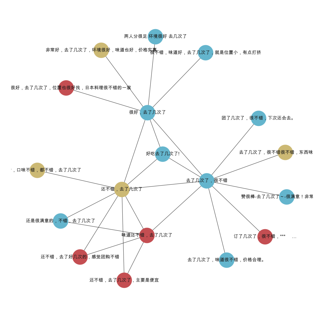
The article is basically over. We can see that we can find a neighbor address for one address, which is quite suitable for mining attempts. However, this algorithm also has certain limitations; the amount of mining cannot be too large. The data we used is relatively small; if the data is large, the mined graph will be even richer. For example, this is based on comments in the course for group mining.
Previous Highlights: