
Author: Huang Yu, Autonomous Driving Scientist
Editor: Hoh Xil
Source: Huang Yu@Zhihu
Produced by: DataFunTalk
Note: There is a latest autonomous driving salon at the end of the article, welcome to sign up.
Introduction: Deep learning has been “hot” for more than ten years since 2006, and the most common applications we see are in computer vision, speech recognition, and natural language processing (NLP). Recently, the industry has been working hard to expand its application scenarios, such as games, content recommendation, and advertisement matching.
Deep learning model architectures can be divided into three types:
❶ Feedforward Networks: MLP, CNN
❷ Feedback Networks: stacked sparse coding, deconvolutional nets
❸ Bidirectional Feedback Networks: deep Boltzmann machines, stacked auto-encoders
Convolutional Neural Networks (CNN) are perhaps the most popular deep learning models and have the greatest impact in computer vision. Below, we introduce the most commonly used CNN models in deep learning and related RNN models, including the famous LSTM and GRU.
—— Basic Concepts ——
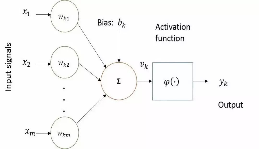
Computational neuroscience has made significant contributions to building computational models of artificial neurons. Artificial neurons that attempt to mimic the behavior of the human brain are the basic building blocks of artificial neural networks. The basic computational elements (neurons) are called nodes (or units), which receive inputs from external sources and have some internal parameters (including weights and biases learned during training) that produce outputs. This unit is called a perceptron. The basic block diagram of a perceptron is shown in the figure below.
The figure shows the basic nonlinear model of a neuron, where 𝑥1, 𝑥2, 𝑥3, … 𝑥𝑚 are input signals; 𝑤𝑘1, 𝑤𝑘2, 𝑤𝑘3, ⋯ 𝑤𝑘𝑚 are synaptic weights; 𝑣𝑘 is the linear combination of input signals; φ (∙) is the activation function (e.g., sigmoid), and 𝑦𝑘 is the output. The offset 𝑏𝑘 is added to the linear combiner of the output, which has the effect of applying an affine transformation, resulting in the output 𝑦𝑘. The function of the neuron can be mathematically represented as follows:
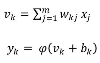
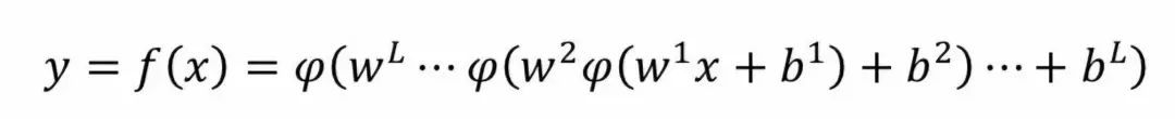
Artificial Neural Networks or general neural networks consist of multiple layers of perceptrons (MLP), containing one or more hidden layers, each with multiple hidden units (neurons). An NN model with MLP is shown in the figure.
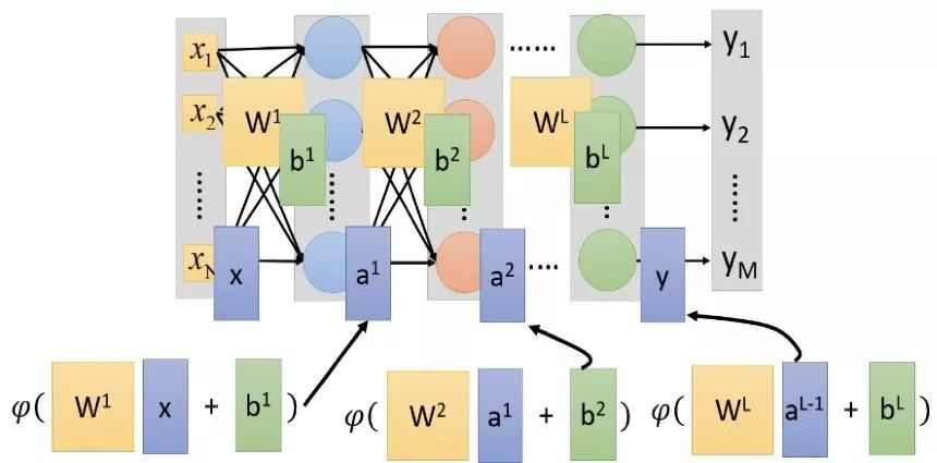
Output of the Multilayer Perceptron:
The learning rate is an important component in training DNNs. It is the step size considered during training, making the training process faster. However, selecting the learning rate is sensitive. If η is too large, the network may start to diverge instead of converge; on the other hand, if η is chosen too small, the network will take longer to converge. Additionally, it may easily get stuck in local minima.
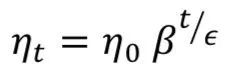
Three common methods can be used to reduce the learning rate during training: constant, factor, and exponential decay. First, a constant ζ can be defined to manually reduce the learning rate based on a defined step function. Second, the learning rate can be adjusted during training according to the following equation:
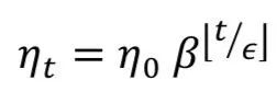
The exponential decay step function format is:
Gradient descent is a first-order optimization algorithm used to find the local minimum of a target function. Algorithm 1 explains the concept of gradient descent:
Algorithm 1 Gradient Descent
Input: Loss function ε, learning rate η, dataset 𝑋, 𝑦 and model F (θ, 𝑥)
Output: Optimal θ that minimizes ε
Repeat until convergence:
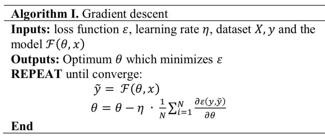
End
Due to the long training time, traditional gradient descent is a major drawback, so the Stochastic Gradient Descent (SGD) method is used to train deep neural networks (DNN). Algorithm 2 explains SGD in detail.
Algorithm 2 Stochastic Gradient Descent
Input: Loss function ε, learning rate η, dataset 𝑋, 𝑦 and model F (θ, 𝑥)
Output: Optimal θ that minimizes ε
Repeat until convergence:
Randomly (𝑋, 𝑦);
For each batch (𝑥i, 𝑦i) of (𝑋, 𝑦) do:
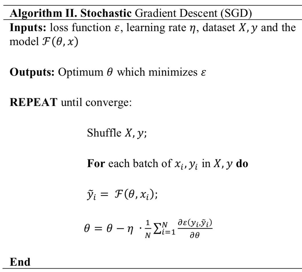
End
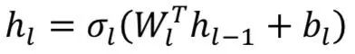
Deep NNs are trained using the popular Backpropagation (BP) algorithm and SGD. Algorithm 3 provides pseudocode for basic BP. In the case of MLP, the NN model can be easily represented using a directed acyclic graph (DAG) such as a computation graph. The representation of DL, as shown in Algorithm 3, allows a single-path network to effectively compute gradients from the top layer to the bottom layer using the chain rule.
Algorithm 3 BP Algorithm
Input: Network with 𝑙 layers, activation function σ𝑙.
Output of hidden layers:
And network output:
Compute gradients:
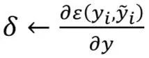
From 𝑖←𝑙 to 0 compute the gradient of the current layer:
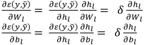
Using  and
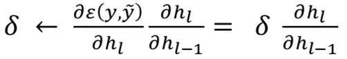
and  Apply gradient descent (GD), backpropagate (BP) gradients to the next layer:
End
Momentum is a method that helps accelerate SGD training. The main idea behind it is to use the moving average of the gradients instead of just the current actual value of the gradients. Its mathematical expression is as follows:
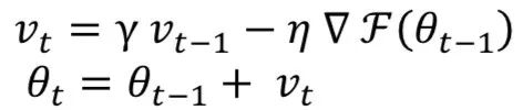
Here, γ is the momentum, and η is the learning rate for the t-th training round. The main advantage of using momentum during training is to prevent the network from getting stuck in local minima. Momentum values are γ∈(0,1). A higher momentum value may make the network unstable. Typically, γ is set to 0.5 until the initial learning stabilizes, then increased to 0.9 or higher.
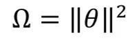
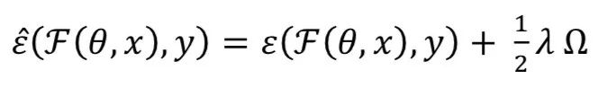
Weight decay is used to train deep learning models as an L2 regularization method, which helps prevent overfitting of the network and model generalization. L2 regularization of F(θ, 𝑥) can be defined as:
The gradient of the weight θ is:
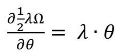
Where 𝜆 = 0.0004.
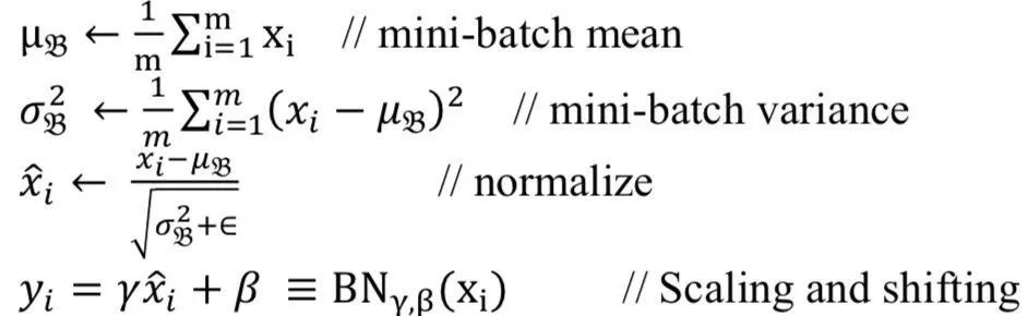
Batch normalization (BN) accelerates the DL process by shifting input samples, which means the input is linearly transformed to zero mean and unit variance. For whitened inputs, the network converges faster and shows better regularization during training, which affects overall accuracy. Since data whitening is performed outside the network, it does not have a whitening effect during model training. In deep Recurrent Neural Networks (RNNs), the input of the n-th layer is a combination of the n-1 layer, not the original feature input. As training progresses, the effects of normalization or whitening decrease, leading to the vanishing gradient problem. This can slow down the entire training process and lead to saturation. To better train, BN is applied to the internal layers of deep neural networks. This method ensures faster convergence in theoretical and benchmark experiments. In BN, the features of one layer are independently normalized to zero mean and variance 1. The algorithm for BN is given in Algorithm 4.
Algorithm 4 BN
Input: Mini-batch (x values): 𝔅= {𝑥1,2,3……,𝑚}
Output: {yi = BNγ, β(xi)}
The activation functions are as follows:
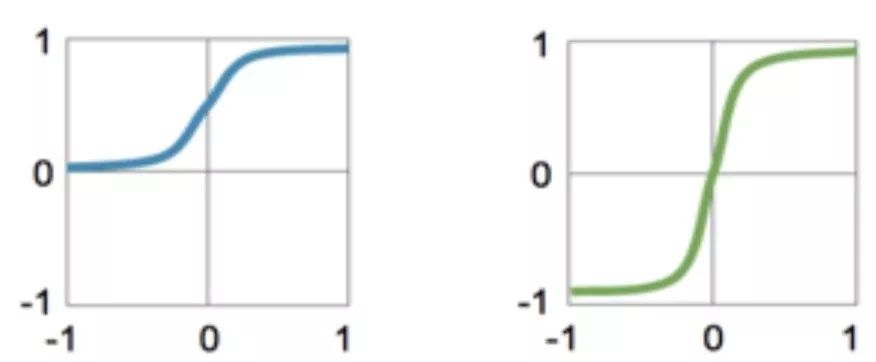
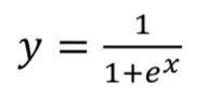
1. Sigmoid
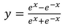
2. TanH
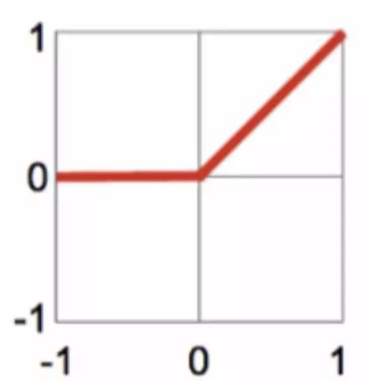
1. Rectified Linear Unit (ReLU): y = max(x, 0)
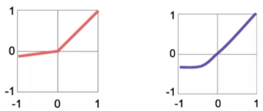
2. Leaky ReLU: y = max(x, ax)
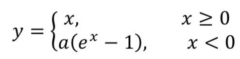
3. Exponential Linear Unit (ELU):
—— Convolutional Neural Networks (CNN) ——
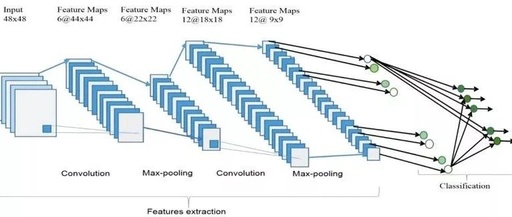
The overall architecture of a CNN is shown in the figure, which includes two main parts: feature extraction and classifier. In the feature extraction layer, each layer of the network receives the output from its previous layer as its input and passes its output as input to the next layer. This CNN architecture is composed of three types of layers: convolution, max-pooling, and classification. There are two types of layers in the lower and middle layers of the network: convolutional layers and max-pooling layers. Even-numbered layers are used for convolution, and odd-numbered layers are used for max-pooling operations. The output nodes of the convolution and max-pooling layers combine to form a 2D plane called a feature map. Each plane of a layer is usually derived from a combination of one or more planes from the previous layer. The nodes of the plane connect to small regions of each connected plane from the previous layer. Each node in the convolutional layer extracts features from the input image through convolution operations. The overall architecture of CNN includes an input layer, multiple alternating convolutional layers and max-pooling layers, a fully connected layer, and a classification layer.

Higher-level features come from features propagated from lower layers. As features propagate to the highest layers or levels, the dimensions of the features decrease depending on the kernel sizes of the convolution and max-pooling operations. However, to ensure classification accuracy, the number of feature maps is usually increased to represent better input image features. The last layer of CNN outputs as input to the fully connected network, which is called the classification layer. Feedforward neural networks have been used as the classification layer.
Relative to the dimensions of the final neural network weight matrix, the expected number of feature selections in the classification layer as input. However, in terms of network or learning parameters, the fully connected layer is expensive. There are several techniques, including average pooling and global average pooling, as alternatives to fully connected networks. In the top classification layer, the softmax layer calculates the scores for the relevant classes. The classifier outputs the relevant class with the highest score.
❶ Convolutional Layer
In this layer, the feature maps from the previous layer are convolved with learnable kernels. The output of the kernels is passed through linear or nonlinear activation functions, such as sigmoid, hyperbolic tangent, softmax, rectified linear, and identity functions, to generate output feature maps. Each output feature map can be combined with multiple input feature maps. Overall, there are
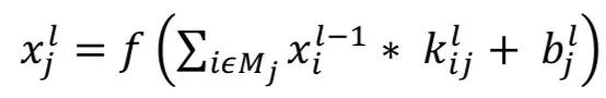
Where 𝑥𝑙 is the output of the current layer, 𝑥𝑙-1 is the output of the previous layer, 𝑘𝑙𝑗𝑖 is the current layer kernel, and 𝑏𝑙𝑗 is the bias of the current layer. 𝑀𝑗 represents the selected input maps. For each output map, an additional bias 𝑏 is provided. However, the input map will be convolved with different kernels to generate the corresponding output maps.
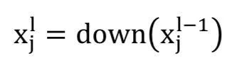
❷ Pooling Layer
The subsampling layer performs downsampling operations on the input maps, which are commonly referred to as pooling layers. In this layer, the number of input and output feature maps does not change. For example, if there are 𝑁 input maps, there will be exactly 𝑁 output maps. Due to the downsampling operation, each dimension size of the output map decreases, depending on the size of the downsampling mask. For example: If a 2×2 downsampling kernel is used, the dimensions of all output maps will be half of the respective input map dimensions. This operation can be expressed as:
Two main types of operations are performed in this layer: average pooling or max pooling. In the average pooling method, the function typically summarizes N×N patches from the feature maps of the previous layer and selects the average value. In max pooling, the highest value is selected from the N×N patches of the feature maps. Therefore, the output map size is reduced by n times. In special cases, the output map is multiplied by a scalar. There are already some alternative subsampling layers, such as fractional max pooling layers and subsampling with convolution.
❸ Classification Layer
This is the fully connected layer that calculates the scores for each class based on the features extracted from the previous convolutional layers. The final layer feature maps are represented as a vector of scalar values, which are passed to the fully connected layer. The fully connected feedforward neural layer serves as the softmax classification layer.
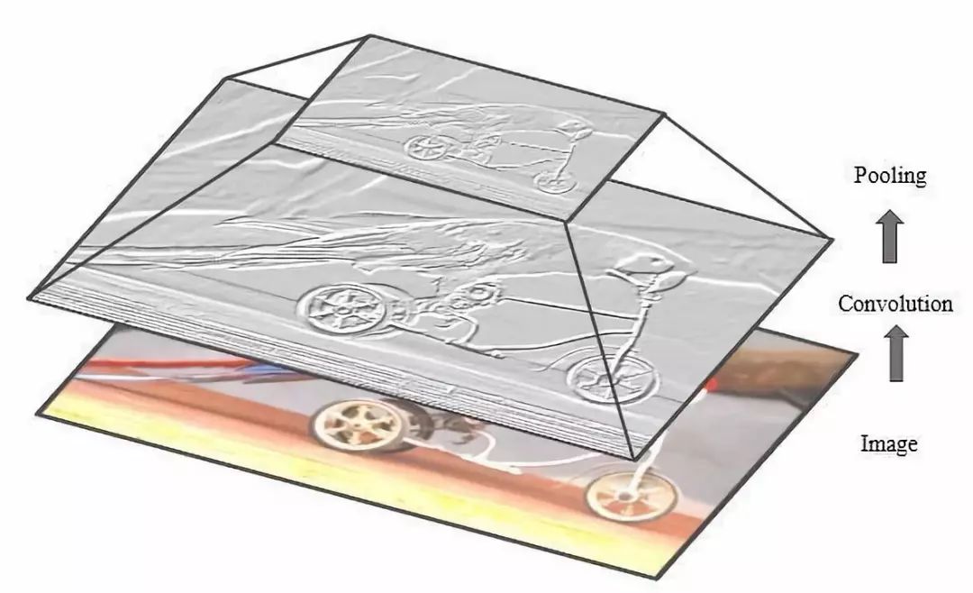
In the backpropagation (BP) of CNN, the fully connected layer is updated according to the methods of fully connected neural networks (FCNN). Full convolution operations are performed on the feature maps between the convolutional layer and its previous layer to update the filters of the convolutional layer. The figure shows the basic operations of convolution and subsampling of the input images.
❹ Network Parameters and Internal Requirements
The number of computed parameters is an important metric for measuring the complexity of deep learning models. The size of the output feature maps:
𝑀= (𝑁-𝐹) /𝑆 +1
Where 𝑁 refers to the size of the input feature maps, 𝐹 refers to the size of the filter or receptive field, 𝑀 refers to the size of the output feature maps, and 𝑆 represents the stride. Padding is usually applied in convolution to ensure that the input and output feature maps have the same size. The number of rows and columns for padding is as follows:
𝑃= (𝐹 – 1) /2
Where 𝑃 is the padding size, and 𝐹 is the kernel dimension. There are several standards to consider when comparing models. However, in most cases, the number of network parameters and memory requirements are considered. The number of parameters for the l-th layer (𝑃𝑎𝑟𝑚𝑙) is calculated according to the following equation:
𝑃𝑎𝑟𝑚𝑙 = (𝐹×𝐹×𝐹𝑀𝑙-1) × 𝐹𝑀𝑙
If the bias is added to the weight parameters, the above equation can be rewritten:
𝑃𝑎𝑟𝑚𝑙 = (𝐹 × (𝐹+1) × 𝐹𝑀𝑙-1) × 𝐹𝑀𝑙
Where the total number of parameters for the l-th layer is denoted as 𝑃𝑙, 𝐹𝑀𝑙 is the total number of output feature maps, and 𝐹𝑀𝑙-1 is the total number of input feature maps or channels. For example, assuming the l-th layer has 𝐹𝑀𝑙-1 = 32 input feature maps, 𝐹𝑀𝑙= 64 output feature maps, and a filter size of 𝐹= 5, in this case, the total number of bias parameters for this layer is:
𝑃𝑎𝑟𝑚𝑙 = (5×5×33) × 64 = 528,000
Thus, the memory size required for the l-th layer operation (𝑀𝑒𝑚𝑙) can be expressed as:
𝑀𝑒𝑚𝑙 = (𝑁𝑙×𝑁𝑙×𝐹𝑀𝑙)
—— Recurrent Neural Networks (RNN) ——
RNNs are unique in that they allow operations over a series of vectors over time. As illustrated in the figure.
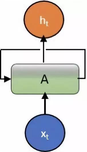
In the Elman architecture, the output of the hidden layer is used together with the normal input of the hidden layer as input. On the other hand, in the Jordan network, the output of the output unit is used as input to the hidden layer. Conversely, Jordan uses the output of the output unit as both its own and the input to the hidden layer. Mathematically, it can be expressed as:
Elman Network:
h𝑡 = 𝜎h(𝑤h𝑥𝑡 + 𝑢hh𝑡−1 + 𝑏h)
𝑦𝑡 = 𝜎𝑦(𝑤𝑦h𝑡 + 𝑏𝑦)
Jordan Network:
h𝑡 = 𝜎h(𝑤h𝑥𝑡 + 𝑢h𝑦𝑡−1 + 𝑏h)
𝑦𝑡 = 𝜎𝑦(𝑤𝑦h𝑡 + 𝑏𝑦)
Where 𝑥𝑡 is the input vector, h𝑡 is the hidden layer vector, 𝑦𝑡 is the output vector, 𝑤 and 𝑢 are weight matrices, and b is the bias vector.
The recurrence allows information to be passed from one step of the network to the next. RNNs can be viewed as multiple copies of the same network, where each network passes messages to its successor. The following diagram shows what happens if the loop is unrolled.
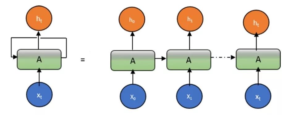
The main problem with the RNN approach is the vanishing gradient.
—— LSTM (Long Short Term Memory) ——
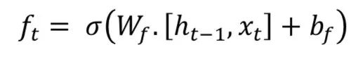
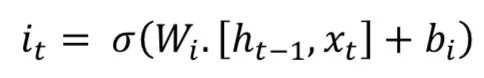
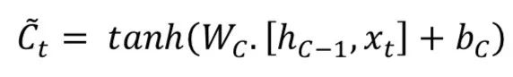
The key idea of Long Short Term Memory (LSTM) is the cell state, as illustrated by the horizontal line running across the top. LSTM removes or adds information to the cell state, called gates: The input gate (𝑖𝑡), forget gate (𝑓𝑡), and output gate (𝑜𝑡) can be defined as follows:
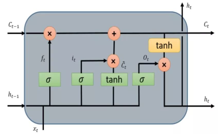
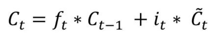
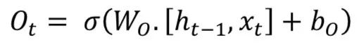
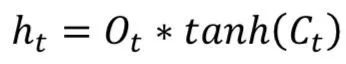
LSTM models are popular in processing temporal information. Most papers containing LSTM models have some slight differences.
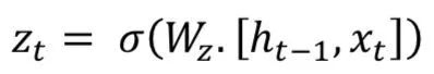
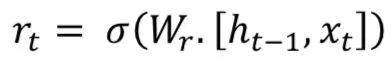
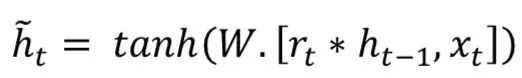
—— Gated Recurrent Unit (GRU) ——
Gated Recurrent Unit (GRU) also comes from LSTMs. The main reason for GRU’s popularity is its computational cost and model simplicity, as shown in the figure. In topology, computational cost, and complexity, GRU is a lighter version of RNN compared to standard LSTM. This technique combines the forget gates and input gates into a single “update gate” and merges cell state, hidden state, and some other variations. Simpler GRU models are becoming increasingly popular. Mathematically, GRU can be represented by the following formula:
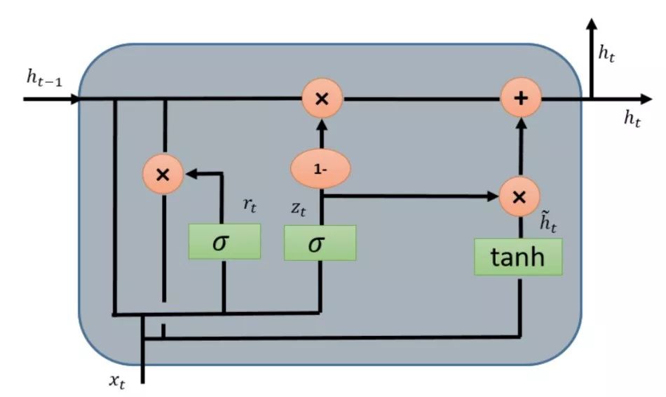
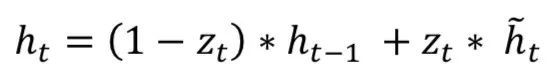
GRU requires fewer network parameters, making the model faster. On the other hand, if there is enough data and computational power, LSTM can provide better performance.
—— References ——
1. https://pathmind.com/wiki/lstm
2. http://colah.github.io/posts/2015-08-Understanding-LSTMs/
3. http://karpathy.github.io/2015/05/21/rnn-effectiveness/
4. M Z Alom et al, “The History Began from AlexNet: A Comprehensive Survey on Deep Learning Approaches”, arXiv 1803.01164, 2018
Original link:
https://zhuanlan.zhihu.com/p/82934581
—— Salon Recommendation ——


Article Recommendation:
Building the Most Reliable Autonomous Driving Infrastructure
Application of Deep Learning in Autonomous Driving Perception

DataFun:
A knowledge-sharing platform focusing on big data and artificial intelligence.

One “look”, one moment!👇