Introduction | Insights from All Courses by Andrew Ng on Deeplearning.ai

The author of this article, Ryan Shrott, Chief Analyst at the National Bank of Canada, has completed all deep learning courses released by Andrew Ng on Coursera to date (as of October 25, 2017) and provides us with insights into the courses.

Among the courses available on Coursera, three are particularly noteworthy:

1. Neural Networks and Deep Learning

2. Improving Deep Neural Networks: Hyperparameter Tuning, Regularization, and Optimization

3. Structuring Machine Learning Projects

I found these three courses to be very important, where we can gain a lot of useful knowledge from Professor Andrew Ng. He does an excellent job with the teaching language, explaining concepts clearly. For example, Andrew Ng clearly states that supervised learning does not go beyond the scope of multi-dimensional curve fitting, and other interpretations of this method, such as simulating the human nervous system, are actually not rigorous.

The prerequisites for these courses are minimal, requiring only some prior knowledge of linear algebra and basic programming in Python. In my opinion, you also need to understand vector calculations to grasp the underlying knowledge of the optimization process. However, if you are not concerned about the internal workings and just want to understand the content at a high level, feel free to skip the calculus part.

Lesson 1: Why is Deep Learning So Popular?

Currently, 90% of the data generated by humans has been collected in the last two years. Deep Neural Networks (DNNs) can leverage massive amounts of data. Therefore, DNNs have surpassed smaller networks and traditional learning algorithms.

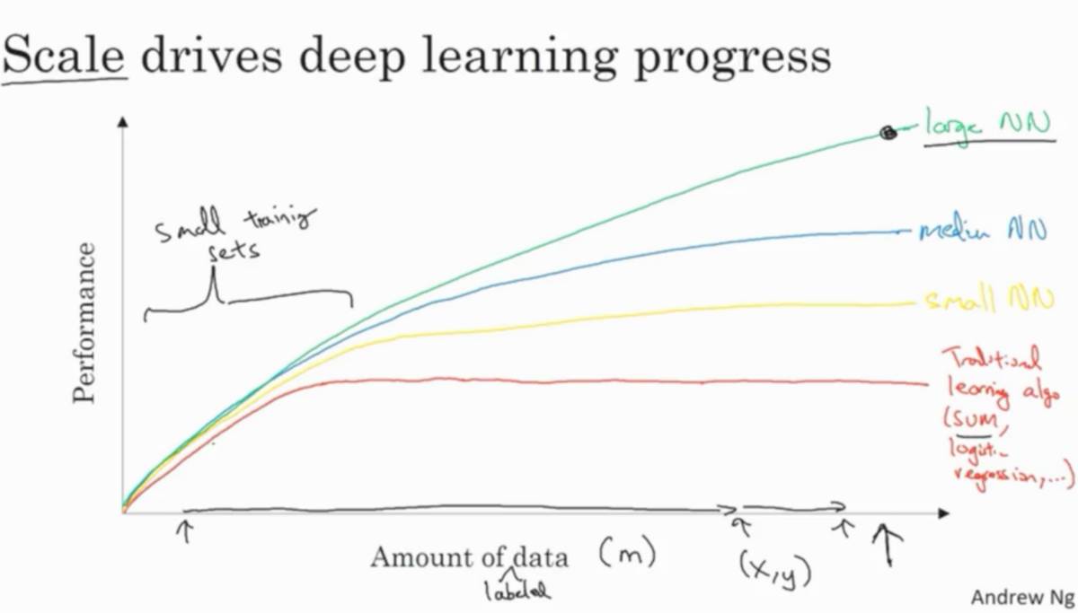
How Scale Drives DNN Performance

Moreover, algorithmic innovations have also accelerated the training speed of DNNs. For instance, switching from the Sigmoid activation function to the ReLU activation function has had a significant impact on the optimization process for tasks like gradient descent. These algorithm improvements allow researchers to traverse the inspiration → code → experience development loop more quickly, leading to more innovation.

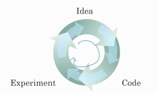
The Deep Learning Development Loop

Lesson 2: Vectorization in Deep Learning

Before starting this lesson, I had no idea that neural networks could be implemented without any explicit loop statements (other than those between layers). Andrew Ng highlights the importance of vectorized programming design in Python. The accompanying assignments guide you to perform vectorized programming, and these methods can be quickly transferred to your own projects.

Lesson 3: Understanding DNNs in Depth

The earlier lessons actually guide you to implement forward and backward propagation from scratch using NumPy. Through this approach, I gained a deeper understanding of how advanced deep learning frameworks like TensorFlow and Keras work. Andrew Ng explains the ideas behind computational graphs, allowing us to understand how TensorFlow achieves “magical optimization”.

Lesson 4: Why Do We Need Depth?

In this section, Andrew Ng explains the concept of layers in DNNs in depth. For example, for a facial recognition system, he explains that the initial processing layers are used to handle facial boundaries, while subsequent layers are used to identify these boundaries as facial components (like nose, eyes, mouth, etc.), and later layers integrate these components to recognize a person’s identity. He also explains the idea of circuit theory—there is a function that requires exponentially many numbers from hidden units to fit the data of shallow networks. The exponential problem can be simplified by adding a limited number of additional layers.

Lesson 5: Tools for Handling Bias and Variance

Andrew Ng explains the steps researchers take to identify and address bias-variance issues. The following diagram illustrates a systematic approach to solving these problems.

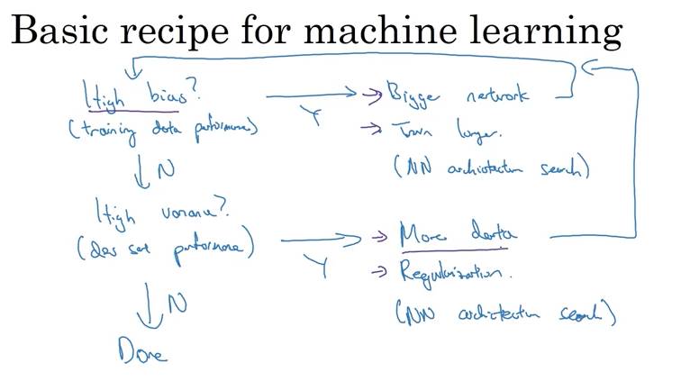
Methods for Addressing Bias and Variance Issues

He also addresses the “tradeoff” between bias and variance. He believes that in today’s era of deep learning, we have independent tools to solve each problem, making tradeoffs no longer exist.

Lesson 6: Regularization

Why does adding a penalty term to the cost function reduce variance? Before taking this course, my understanding was that it brings the weight matrix closer to zero, resulting in a more “linear” function. Andrew Ng provides another explanation related to the tanh activation function, where smaller weight matrices generate smaller outputs, keeping the outputs centered around the linear region of the tanh function.

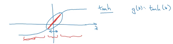
tanh Activation Function

He also provides an interesting explanation of dropout. Previously, I thought dropout randomly eliminates neurons in each iteration, similar to how a smaller network has a stronger linearity. However, Andrew Ng’s explanation views it from the perspective of individual neurons’ lives.

Perspective of Individual Neurons

Since dropout randomly eliminates connections, it encourages neurons to distribute weights more evenly among parent neurons. By expanding weights, it can reduce the L2 norm (squared norm) of weights. He also explains that dropout is an adaptive form of L2 regularization, and the two methods yield similar results.

Lesson 7: Why Normalization Works?

Andrew Ng demonstrates why normalization can accelerate optimization steps by plotting contour maps. He explains in detail the variations in the number of iterations required for gradient descent on normalized versus non-normalized contour maps, indicating that the same optimization algorithm without normalization requires more iterations.

Lesson 8: The Importance of Initialization

Andrew Ng states that not using parameter initialization can lead to vanishing or exploding gradients. He shows multiple steps to address these issues. The basic principle is to ensure that the variance of the weight matrix for each layer is approximately 1. He also discusses Xavier initialization for the tanh activation function.

Lesson 9: Why Use Mini-Batch Gradient Descent?

Andrew Ng uses contour maps to explain the trade-offs between using mini-batch and large-batch training. The basic principle is that larger batches slow down each iteration while smaller batches can speed up the iteration process but do not guarantee the same convergence effect. The best approach is to find a balance between the two, making the training process faster than processing the entire dataset at once while leveraging the advantages of vectorization techniques.

Lesson 10: Intuitive Understanding of Advanced Optimization Techniques

Andrew Ng explains how to appropriately use techniques like momentum and RMSprop to limit the paths of gradient descent approaching the minima. He vividly illustrates this process with the example of a ball rolling down a hill. He combines these methods to explain the famous Adam optimizer.

Lesson 11: Basic Understanding of the TensorFlow Backend

Andrew Ng not only explains how to use TensorFlow to implement neural networks but also discusses the backend processes that occur during optimization. One of the assignments encourages us to implement dropout and L2 regularization using TensorFlow, which deepens my understanding of the backend processes.

Lesson 12: Orthogonalization

Andrew Ng also discusses the importance of regularization in machine learning strategies. The basic idea is that we want to implement and control the factors affecting algorithm performance, controlling only one factor at a time. For example, to address bias issues, we can use larger networks or more robust optimization techniques, and we want these controls to only affect bias without impacting other issues like generalization. A case lacking orthogonal control is prematurely stopping the optimization process of the algorithm, as this would simultaneously affect both the model’s bias and variance.

Lesson 13: The Importance of Single Number Evaluation Metrics

Andrew Ng emphasizes the importance of choosing a single number evaluation metric, which allows us to evaluate algorithms. If the goal changes, we should only change the evaluation metric during the model development process. Andrew Ng illustrates this with a case of using a cat classification application to identify explicit images.

Lesson 14: Distribution of Test and Development Sets

We usually assume that the distribution of the test set is the same as that of the development set (dev sets), ensuring that we are optimizing towards the right target during the iteration process. This also means that if you decide to correct mislabelled data in the test set, you need to correct the mislabelled data in the development set as well.

Lesson 15: Handling Different Training and Testing/Development Distributions

Andrew Ng introduces why we are interested in the issue of having different distributions for training and testing/development sets. This is because we want to calculate evaluation metrics based on samples that are actually of concern. For example, we may want to train using samples that are irrelevant to the training problem, but we do not want the algorithm to use these samples for evaluation, allowing our algorithm to train on more data. Empirically, this approach can yield very good results in many cases. The downside is that our training and testing/development sets may have different distributions. A common solution to this problem is to set aside a small portion of the training set and determine the generalization performance of the training set. We can then compare these error rates with the actual development error and calculate a metric for “data mismatch.” Andrew Ng also explains methods for addressing these data mismatch issues, such as synthetic data generation.

Lesson 16: Size of Training/Development/Test Sets

In the era of deep learning, the methods for separating training/development/test sets have also undergone significant changes. Previously, I only knew the common 60/20/20 split. Andrew Ng emphasizes that for a very large dataset, a split of 98/1/1 or even 99/0.5/0.5 should be used. This is because as long as the development and test sets are large enough to ensure that the model is within the confidence interval set by the team, it is sufficient. If you use 10 million training samples, then 100,000 samples (1% of the dataset) are enough to ensure the confidence interval for the development and/or test set.

Lesson 17: Approximate Bayesian Optimal Error

Andrew Ng explains how human-level performance in certain applications serves as a substitute for Bayesian error. For instance, in visual and auditory recognition tasks, human-level error is often very close to Bayesian error and can be used to quantify the avoidable bias in models. Without benchmarks like Bayesian error, understanding variance and avoidable bias issues in networks is quite difficult.

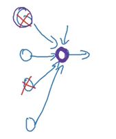
Lesson 18: Error Analysis

Andrew Ng introduces an effective error analysis technique that can significantly improve algorithm performance. The basic idea is to manually label misclassified samples and focus on addressing the errors that most impact the misclassified data.

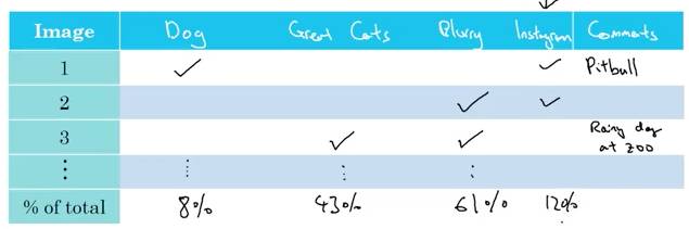
Error Analysis of Cat Recognition App

For example, in cat recognition, Andrew Ng believes that blurry images are the easiest to misclassify. This sensitivity analysis can show how worthwhile your efforts are in reducing overall error. Another possibility is that fixing blurry images is a labor-intensive task, while other errors are easier to understand and fix. Sensitivity analysis and approximate operations will factor into the decision-making process.

Lesson 19: When to Use Transfer Learning?

Transfer learning allows knowledge from one model to be transferred to another. For example, you can transfer image recognition knowledge from a cat recognition app to radiology diagnostics. Implementing transfer learning requires retraining the last few layers of the network with more data for similar application domains. The underlying idea is that the lower-level hidden units of the network have a broader range of applications, meaning they are not sensitive to specific task types. In summary, transfer learning is feasible when tasks share the same input features and the task requiring learning has much more data than the task requiring training.

Lesson 20: When to Use Multi-Task Learning?

Multi-task learning forces a single neural network to learn multiple tasks simultaneously (as opposed to configuring a separate neural network for each task). Andrew Ng explains that this method works well when the task set gains learning benefits by sharing lower-level features, and the data scales for each task are similar.

Lesson 21: When to Use End-to-End Deep Learning?

End-to-end deep learning requires multiple layers of processing combined into a single neural network, allowing data to autonomously undergo an optimization process without introducing bias from manually designed steps. On the other hand, this method requires a lot of data, which may exclude potential manual design components.

Conclusion

Andrew Ng’s deep learning courses have given me a basic intuitive understanding of the development process of deep learning models. The courses I have explained above are just a portion of the materials presented in this course. Even after completing the course, you cannot yet call yourself a deep learning expert, and my only dissatisfaction is that the assignments are too simple. By the way, writing this article did not receive approval from deeplearning.ai.

Original link: https://medium.com/towards-data-science/deep-learning-specialization-by-andrew-ng-21-lessons-learned-15ffaaef627c

This article is translated by Machine Heart, Please contact this public account for authorization.

✄————————————————

Join Machine Heart (Full-time Reporter/Intern): [email protected]

Submissions or Seeking Coverage: [email protected]

Advertisement & Business Cooperation: [email protected]