
Source: Machine Heart
This article contains 3744 words, and is recommended for a reading time of 8 minutes. Through this article, we will explain how to build models for natural language, audio, and other sequential data.
Since Andrew Ng released the deeplearning.ai courses, many learners have completed all the specialized courses and meticulously created course notes. Last month, the fifth course of deep learning.ai was released, marking the end of this series of courses. Mahmoud Badry has open-sourced the complete notes for all five courses on GitHub, detailing knowledge points including sequence models. We briefly introduce this project and focus on the sequence model from the fifth course.
Project address: https://github.com/mbadry1/DeepLearning.ai-Summary
Last week, Andrew Ng showcased an infographic completed by TessFerrandez on Twitter, beautifully documenting the knowledge and highlights of the deep learning courses. For a detailed introduction to this infographic, see: This deep learning course note was praised by Andrew Ng.
The deeplearning.ai courses have been continuously followed since their launch, and many readers have actively participated in the learning process. The notes completed by Mahmoud Badry are mainly divided into five parts, corresponding to the basics of neural networks and deep learning, techniques and methods to enhance DNN performance, structured machine learning projects, convolutional neural networks, and sequence models. It is worth noting that the notes for this project are very detailed, covering almost all knowledge points of the five courses. For example, the first course records basic knowledge points from an introduction to neural networks to an interview with Goodfellow, organized by different themes each week.
Since many knowledge points from the first four courses have already been introduced, this article will focus on summarizing the notes from the fifth course, and readers can refer to GitHub to read the complete notes.
Introduction to the Fifth Course: Sequence Models
This course will teach how to build models for natural language, audio, and other sequential data. With the help of deep learning, sequence algorithms perform better than they did two years ago and are used in many interesting applications such as speech recognition, music synthesis, chatbots, machine translation, and natural language understanding. By the end of this course, you will:
-
Understand how to build and train recurrent neural networks (RNNs) and their common variants, such as GRU and LSTM.
-
Use sequence models to handle natural language problems, such as text synthesis.
-
Apply sequence models to audio applications, such as speech recognition and music synthesis.
-
This is the fifth and final course of the Deep Learning Specialization.
Target Audience:
-
Learners who have completed the first, second, and fourth courses. It is also recommended to study the third course.
-
Individuals who have a deep understanding of neural networks (including CNNs) and wish to learn how to develop recurrent neural networks.
This course introduces recurrent neural networks (RNNs), natural language processing, word embeddings, sequence models, and attention mechanisms. Below is a brief introduction to the sequence model notes completed by Mahmoud Badry.
Sequence Models:
Sequence models (such as RNNs and LSTMs) have greatly transformed sequence learning, and they can be enhanced through attention mechanisms. Sequence models are applied in areas such as speech recognition, music generation, sentiment classification, DNA sequence analysis, machine translation, video activity recognition, and named entity recognition.
Recurrent Neural Network Model (RNN)
Recurrent neural networks emerged in the 1980s and have recently gained popularity due to advancements in network design and increased computational power on graphics processing units. This type of network is particularly useful for sequential data because each neuron or unit can use its internal memory to retain relevant information from previous inputs. In the case of language, the sentence “I had washed my house” has a different meaning than “I had my house washed.” This allows the network to gain a deeper understanding of the expression.
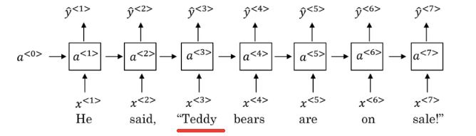
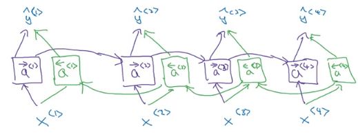
RNNs have many applications and perform well in the field of natural language processing (NLP). The following image shows an RNN network used for named entity recognition tasks.
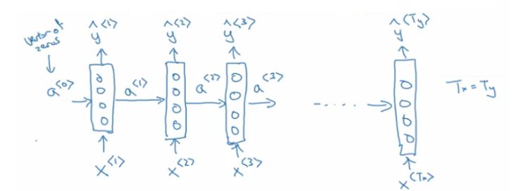
RNN network used for named entity recognition tasks.
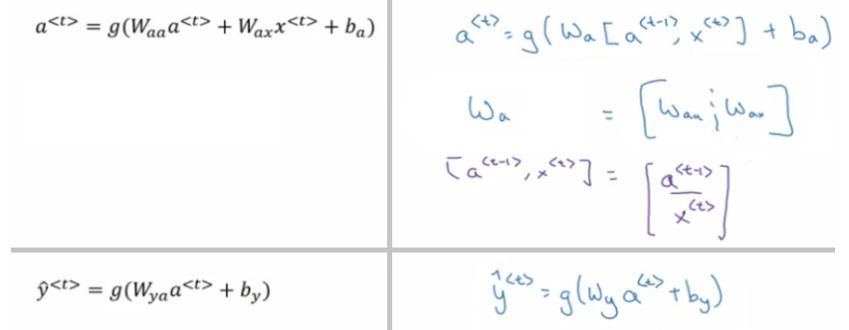
Simplified representation of RNN.
Backpropagation Through Time (BPTT)
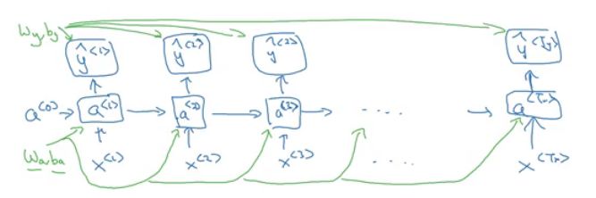
Backpropagation in RNN architecture, where w_a, b_a, w_y, b_y are shared across all elements in the sequence.
Here, we use the cross-entropy loss function:
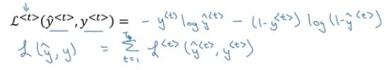
The first formula represents the loss function for one element in the sequence, while the total loss for the entire sequence is the sum of each element’s loss.
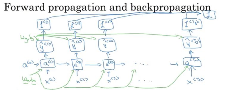
In the above image, the activation value a propagates from one sequence element to another.
Types of RNNs
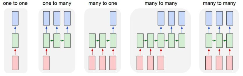
Different types of RNNs.
Gradient Vanishing in RNNs
Gradient vanishing refers to the phenomenon where the gradient norm of parameters decreases exponentially as network depth increases. A small gradient means slow parameter changes, which can stall the learning process. While RNNs have strong capabilities in sequence problems like language modeling, they also face severe gradient vanishing issues. Therefore, gated RNNs such as LSTM and GRU have great potential, as they use gating mechanisms to retain or forget information from earlier time steps and form memories for the current computation process.
Gated Recurrent Unit (GRU)
GRUs are designed to address the gradient vanishing problem that occurs in standard RNNs. The principles behind GRUs are very similar to those of LSTMs, using gating mechanisms to control the input, memory, and other information to make predictions at the current time step, expressed as follows:
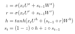
GRUs have two gates: a reset gate and an update gate. Intuitively, the reset gate determines how to combine new input information with previous memory, while the update gate defines how much of the previous memory is retained for the current time step. If we set the reset gate to 1 and the update gate to 0, we will obtain the standard RNN model again. The fundamental idea of using gating mechanisms to learn long-term dependencies is consistent with LSTMs, but there are some key differences:
-
GRUs have two gates (reset gate and update gate), while LSTMs have three gates (input gate, forget gate, and output gate).
-
GRUs do not control and retain internal memory (c_t) and do not have an output gate like LSTMs.
-
The input and forget gates in LSTMs correspond to the update gate in GRUs, while the reset gate directly affects the previous hidden state.
-
Second-order nonlinearity is not applied when computing the output.
To solve the gradient vanishing problem in standard RNNs, GRUs use the update gate and reset gate. Essentially, these two gating vectors determine which information can ultimately be output as a gated recurrent unit. The uniqueness of these two gating mechanisms lies in their ability to retain information over long sequences without being cleared over time or removed due to irrelevance to predictions.
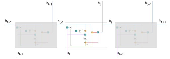
Recurrent neural network with gated recurrent units
Below is the specific structure of a single gated recurrent unit.
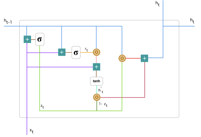
Gated recurrent unit
LSTM
Using traditional backpropagation through time (BPTT) or real-time recurrent learning (RTTL), the error signals flowing backward through time often explode or vanish. However, LSTMs can reduce these issues through mechanisms for forgetting and retaining memory.
LSTM units typically output two states to the next unit: the cell state and the hidden state. The memory block is responsible for remembering the hidden states or events from previous time steps, and this memory is generally implemented through three gating mechanisms: the input gate, forget gate, and output gate.
Below is the detailed structure of an LSTM unit, where Z is the input part, and Z_i, Z_o, and Z_f are the values that control the three gates, filtering the input information through the activation function f. The activation function is typically chosen to be the Sigmoid function, as its output value ranges from 0 to 1, indicating the extent to which these three gates are opened.
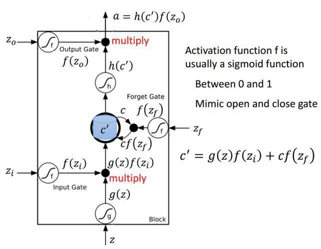
Image source: Li Hongyi’s Machine Learning Lecture Notes.
If we input Z, then the input vector’s output g(Z) multiplied by the input gate f(Z_i) represents the information retained after filtering. The forget gate controlled by Z_f determines how much of the previous memory is retained, which can be represented by the equation c*f(z_f). The useful information from the previously retained memory combined with the meaningful information from the current input will be retained for the next LSTM unit, which we can express as c’ = g(Z)f(Z_i) + cf(z_f), where the updated memory c’ represents all useful information retained from the past and present. We then take the activation value of this updated memory h(c’) as the potential output, which can typically be chosen to use the tanh activation function. Finally, the remaining part is controlled by the output gate Z_o, which determines which activated outputs from the current memory are useful. Therefore, the final output of the LSTM can be expressed as a = h(c’)f(Z_o).
Bidirectional RNN (BRNN)
Bidirectional RNNs and deep RNNs are effective methods for building powerful sequence models. The following image shows an RNN model for a named entity recognition task:
BRNN Architecture
The downside of BRNNs is that they require the entire sequence to be processed beforehand.
Deep RNN
Deep RNNs can help build powerful sequence models.
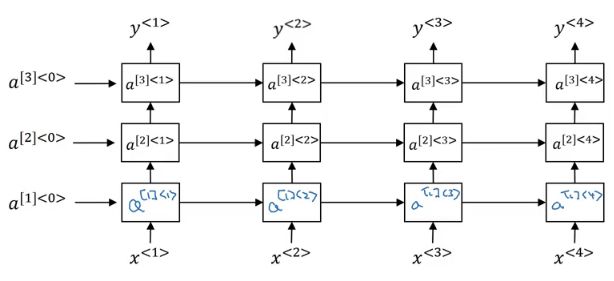
Illustration of a 3-layer deep RNN.
Backpropagation in RNNs
In modern deep learning frameworks, you only need to implement forward propagation, and the framework will perform backpropagation, so most machine learning engineers do not need to worry about backpropagation. However, if you are a calculus expert and want to understand the details of backpropagation in RNNs, you can refer to this notebook: https://www.coursera.org/learn/nlp-sequence-models/notebook/X20PE/building-a-recurrent-neural-network-step-by-step.
Natural Language Processing and Word Representation
Word representation is an essential part of natural language processing. From the early One-Hot encoding to the now popular word embeddings, researchers have been searching for efficient methods of word representation. Mahmoud Badry has recorded the methods of word embedding in detail in his notes, including word embeddings used for named entity recognition, face recognition, and translation systems. The following image shows the structure of word embeddings used for face recognition:
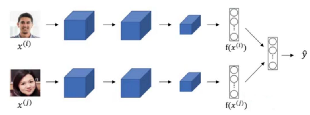
In this word embedding method, we can compress different face encodings into a vector, allowing us to compare whether they represent the same face.
Word embeddings have many excellent properties. For instance, given a word embedding table, this note explains the semantic similarity of word embeddings through cases. As shown in the following image, the transformation from male to female is the same as that from king to queen in the embedding space, indicating that word embeddings capture the semantic relationships between words.
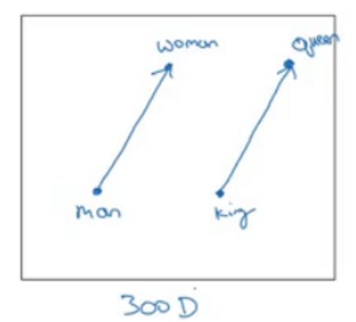
Generally speaking, the Word2Vec method consists of two parts. First, it maps words represented in high-dimensional one-hot form to low-dimensional vectors. For example, converting a matrix with 10,000 columns into one with 300 columns is called word embedding. The second goal is to retain the meaning of words while preserving their context to some extent. Word2Vec achieves these two goals through methods such as skip-gram and CBOW. The skip-gram model inputs a word and attempts to estimate the probability of other words appearing near that word. The opposite method is called Continuous Bag Of Words (CBOW), which uses some context words as input and finds the word that best fits (with the highest probability) that context.
For the Continuous Bag Of Words model, Mikolov and others used the n words before and after the target word to predict it simultaneously. They called this model the Continuous Bag Of Words (CBOW) because it represents words in continuous space, where the order of these words is not important. CBOW can be seen as a language model with foresight, while the skip-gram model completely changes the objective of the language model: instead of predicting the middle word from surrounding words like CBOW, it predicts surrounding words from the center word.
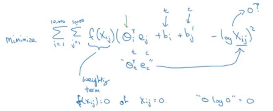
Mahmoud Badry also demonstrated another method for learning word embeddings called GloVe, which, although not as widely used as language models, has a streamlined structure that is very easy to understand:
Sequence Models and Attention Mechanisms
The final section focuses on attention mechanisms, including the shortcomings of encoder-decoder architectures and the solutions introduced by attention mechanisms. The following image illustrates the process of encoding information using context vectors C or attention weights.
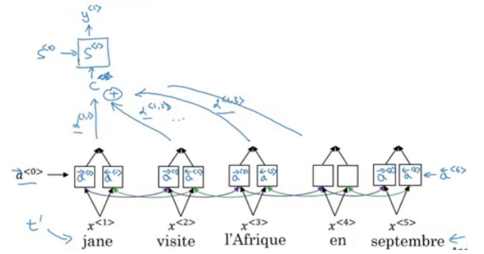
When we translate a sentence, we particularly focus on the word being translated. Neural networks can achieve the same behavior through attention, focusing on a subset of the received information.
We typically use context-based attention to generate attention distributions. The participating RNN generates a query that describes what it wants to focus on. Each entry is dot-multiplied with this query to produce a score that describes the degree of match between this entry and the query. These scores are input into a softmax to generate the attention distribution.