Follow the public account “ML_NLP”

Set as “Starred”, heavy content delivered first time!

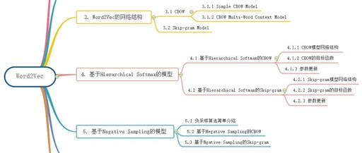
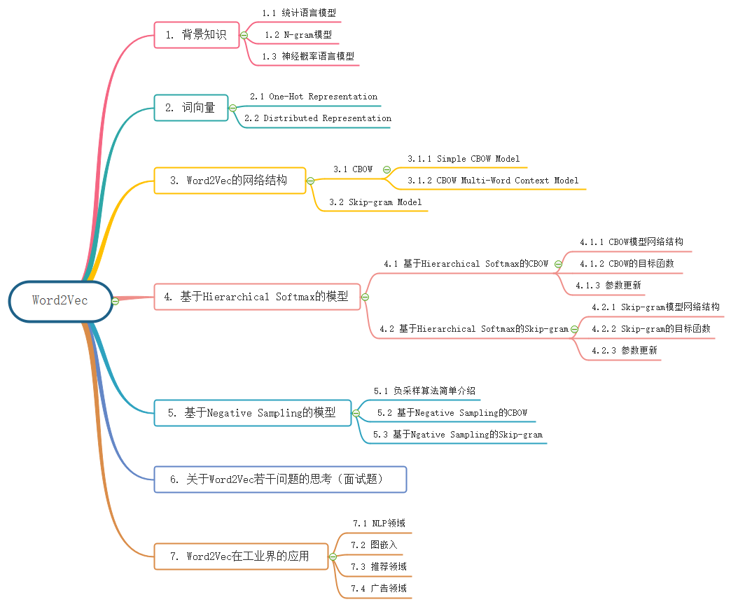
Overview of this article:

1. Background Knowledge

Word2Vec is a type of language model that learns semantic knowledge from a large amount of text data in an unsupervised manner, and is widely used in natural language processing.

Word2Vec is a tool for generating word vectors, which are closely related to language models. Therefore, we will first understand some knowledge related to language models.

1.1 Statistical Language Models

A statistical language model is a probabilistic model used to calculate the probability of a sentence, usually based on a corpus. So what does it mean to calculate the probability of a sentence? Suppose that a sentence is composed of words in order, and the joint probability of the sentence is:

This is called a language model, which is used to calculate the probability of this sentence. Using Bayes’ theorem, the above can be decomposed into:

Where the conditional probability is the parameter of the language model. If all these parameters are calculated, then given a sentence, the corresponding probability can be quickly calculated.

It seems simple, right? However, the specific implementation is still a bit tricky. For example, let’s first look at the number of model parameters. Just now, we considered a given sentence of length T, which requires calculating T parameters. Assuming the size of the vocabulary corresponding to the corpus is V, then if we consider sentences of any length n, theoretically there are V^n possibilities, and each possibility requires calculating V parameters, totaling V^(n*T) parameters. Of course, this is just a rough estimate and does not consider duplicate parameters, but this magnitude is still a bit scary. In addition, after calculating these probabilities, they also need to be stored, so storing this information also requires a large memory overhead.

Furthermore, how are these parameters calculated? Common methods include n-gram models, decision trees, maximum entropy models, maximum entropy Markov models, conditional random fields, neural networks, and more. This article will only discuss n-gram models and neural networks.

1.2 N-gram Models

Consider the approximate calculation of P(W_n | W_1, W_2, …, W_{n-1}). Using Bayes’ theorem, we have:

According to the law of large numbers, when the corpus is large enough, P(W_n | W_1, W_2, …, W_{n-1}) can be approximately represented as:

Where C(W_n) represents the number of times the word sequence W_n appears in the corpus, and C(W_1, W_2, …, W_{n-1}) represents the number of times the word sequence W_1, W_2, …, W_{n-1} appears in the corpus. It can be imagined that when n is large, the statistics of C(W_n) and C(W_1, W_2, …, W_{n-1}) will be very time-consuming.

From formula (1), it can be seen that the probability of a word appearing is related to all the previous words. If we assume that the probability of a word appearing is only related to a fixed number of previous words, this is the basic idea of the n-gram model, which makes a Markov assumption of order k, asserting that the probability of a word appearing is only related to the previous k words, that is,

Then, formula (2) becomes:

For example, if k=2, we have:

This simplification not only makes the statistics of individual parameters easier (the word sequences to match during statistics become shorter), but also reduces the total number of parameters.

So, what should be the appropriate size of k in n-gram? Generally speaking, the choice of k needs to consider both computational complexity and model performance.

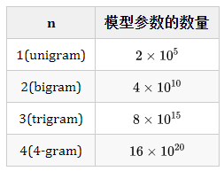
Table 1: Relationship Between Model Parameter Count and k

In terms of computational complexity, Table 1 shows how the number of model parameters in the n-gram model changes as k increases, assuming the vocabulary size is V (the vocabulary size of Chinese is roughly of this magnitude). In fact, the magnitude of model parameters is an exponential function of k (O(V^k)), and obviously k cannot be too large; in practical applications, at most a trigram model is used.

In terms of model performance, theoretically, the larger k is, the better the performance. Nowadays, the vast amount of data on the internet and improvements in machine performance make it possible to compute higher-order language models (such as k>3), but it should be noted that when k reaches a certain level, the performance improvement will diminish. For example, when increasing from k=2 to k=3, the performance improves significantly, while increasing from k=3 to k=4 does not show significant improvement (for specifics, refer to related chapters in Wu Jun’s book “The Beauty of Mathematics”). In fact, this also involves a trade-off between reliability and distinguishability; the more parameters there are, the better the distinguishability, but at the same time, the fewer instances of each parameter, which reduces reliability, so a balance must be struck between reliability and distinguishability.

Additionally, there is an important step called smoothing in the n-gram model. Returning to formula (3), consider two questions:

• If C(W) = 0, can we consider P(W) to be equal to 0?
• If C(W) = 1, can we consider P(W) to be equal to 1?

Clearly, this cannot be the case, but it is an unavoidable problem, no matter how large your corpus is. Smoothing techniques are used to address this issue, which will not be elaborated on here.

In summary, the n-gram model is a model primarily focused on counting the occurrences of various word sequences in the corpus and smoothing. Once the probability values are calculated, they are stored, and when calculating the probability of a sentence next time, it is sufficient to find the corresponding probability parameters and multiply them together.

However, in the field of machine learning, there is a universal method for solving problems: after modeling the problem at hand, first construct an objective function for it, then optimize that objective function to obtain a set of optimal parameters, and finally use the model corresponding to this set of optimal parameters for prediction.

For statistical language models, using maximum likelihood, we can set the objective function as:

Where C represents the corpus, and W represents the context of the word, i.e., the set of surrounding words. When W is empty, we take P(W). Specifically, for the previously introduced n-gram model, we have P(W_n | W_1, W_2, …, W_{n-1}).

Of course, in practical applications, maximum log likelihood is often used, that is, setting the objective function as:

Then maximizing this function.

From formula (4), it can be seen that the probability P has been treated as a function of W and W_n, that is:

Where θ is the set of parameters to be determined. In this way, once the optimal parameter set θ is obtained by optimizing formula (4), it is uniquely determined, and any probability can be calculated through the function P.

Compared with n-gram, this method does not require pre-calculation and storage of all probability values; instead, it obtains them through direct computation, and by selecting an appropriate model, the number of parameters in θ can be far less than that in the n-gram model.

Clearly, the most critical aspect of such a method is the construction of the function. The next section will introduce a method of construction using neural networks. This method is specifically introduced because it can be seen as the predecessor or foundation of the algorithm framework in Word2Vec.

1.3 Neural Probabilistic Language Model

This section introduces a neural probabilistic language model proposed by Bengio et al. in their 2003 paper “A Neural Probabilistic Language Model.” This paper was the first to propose using neural networks to solve the problem of language modeling. Although it did not receive much attention at the time, it laid a solid foundation for later deep learning in solving language modeling problems and many other NLP issues. Future researchers built upon the work of Yoshua Bengio and achieved further accomplishments, including Tomas Mikolov, the author of Word2Vec, who proposed RNNLM and later Word2Vec based on NNLM. The paper also early proposed representing words as low-rank vectors instead of One-Hot. Word embedding, as a byproduct of a language model, played a crucial role in subsequent research, providing researchers with a broader perspective. It is worth noting that the concept of Word2Vec was also proposed in this paper.

What is a word vector? Simply put, for any word in the vocabulary, a fixed-length real-valued vector is assigned, which is called the word vector of that word. The length of the word vector is denoted as d. Further understanding of word vectors will be discussed in the next section.

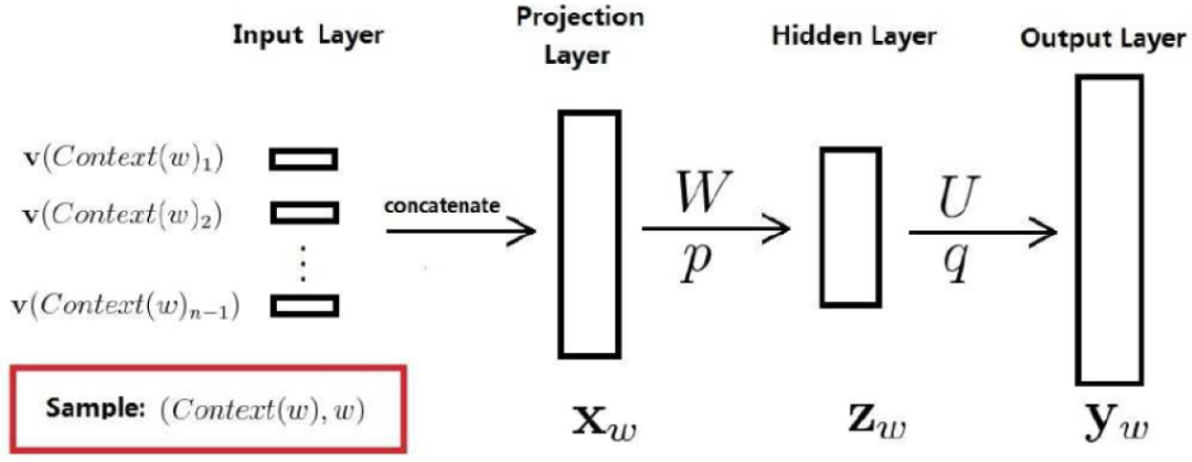
Since it is a neural probabilistic language model, neural networks must be used. The diagram below shows the structure of the neural network. The model consists of three layers: the first layer is the mapping layer, which maps the words to their corresponding word embeddings; this layer is actually the input layer of the MLP; the second layer is the hidden layer, using a specific activation function; the third layer is the output layer, which, since it is a language model, needs to predict the next word based on the previous words, thus it is a multi-class classifier. The largest computation of the entire model is concentrated in the last layer since, generally speaking, the vocabulary is large, requiring the calculation of the conditional probability of each word, which becomes the computational bottleneck of the entire model.

The result obtained from the calculations above is just a vector of length d, whose components cannot represent probabilities. If we want the components of this vector to represent the probability of the next word being the nth word given the context, we need to perform a Softmax normalization, after which it can be represented as:

Where index n represents the index of the word in the vocabulary.

Here, it is necessary to initialize a word embedding matrix in advance, where each row represents the vector of a word. The word vectors are also training parameters that are updated during each training iteration. Here we can see that word vectors are a byproduct of the language model, as the work of the language model itself is to estimate how human-like a given sentence is, but subsequent research found that language models have become a very good tool.

Softmax is a very inefficient processing method, requiring the calculation of the probability of each word and also the exponentiation, which is computationally expensive. Many subsequent studies have optimized this problem, such as hierarchical softmax and softmax trees.

Of course, NNLM’s performance may not seem impressive by today’s standards, but it is of great importance for subsequent related research. The paper’s Future Work section mentioned that using RNN instead of MLP as the model might yield better results, which was later validated in Tomas Mikolov’s doctoral thesis, leading to RNNLM.

What advantages does the neural probabilistic language model have compared to the n-gram model? There are mainly two points:

• The similarity between words can be reflected through word vectors.

For example, if a certain word appears 10 times in a corpus, and another word appears only 2 times, according to the n-gram model, the probability of the first word will be much larger than that of the second. However, the only difference between the two words is that one is “dog” and the other is “cat,” and both play similar roles syntactically and semantically; therefore, their probabilities should be very close. In fact, the probabilities calculated by the neural probabilistic language model for these two words are roughly equal. The reason is that (1) in the neural probabilistic language model, it is assumed that the word vectors of “similar” words are also similar; (2) the probability function regarding word vectors is smooth, meaning that a small change in the word vector will only lead to a small change in probability. Thus, for the following sentences, as long as one appears in the corpus, the probabilities of the others will also increase accordingly.

A dog is running in the room. A cat is running in the room. The cat is running in a room. A dog is walking in a bedroom. The dog was walking in the room.

• The model based on word vectors has a built-in smoothing function (as shown in formula (5), P(W) will not be zero), eliminating the need for additional processing like n-gram models.

Finally, let’s think about what role word vectors play in the entire neural probabilistic language model. During training, they serve as auxiliary parameters to help construct the objective function, and after training, they seem to be just a byproduct of the language model. But this byproduct should not be underestimated, and the next section will elaborate further on it.

2. Word Vectors

In natural language processing tasks, natural language needs to be processed by machine learning algorithms, which usually requires mathematical representation of language, as machines do not understand human language but only recognize mathematical symbols. Vectors are the abstraction of real-world entities that humans provide for machines to process, and it can be said that vectors are the main way humans input data to machines.

Word vectors are a way to mathematically represent words in language; as the name suggests, a word vector represents a word as a vector. We know that words need to be encoded into numerical variables before being fed into neural network training. Common encoding methods include One-Hot Representation and Distributed Representation.

2.1 One-Hot Representation

One of the simplest word vector methods is One-Hot encoding, which uses a long vector to represent a word, with the length equal to the size of the vocabulary. The vector has only one 1, and all other elements are 0, with the position of 1 corresponding to the word’s position in the vocabulary.

For example: I like writing code. The One-Hot encoding would be:

Word	One-Hot Encoding
I	1 0 0 0
like	0 1 0 0
writing	0 0 1 0
code	0 0 0 1

This One-Hot encoding can be very compact if stored in a sparse way: that is, assigning each word a numeric ID. For example, in the above case, “code” is assigned ID 3, and “like” is assigned ID 2. If you want to implement this programmatically, you can use a hash table to assign a number to each word. Such a compact representation, combined with algorithms like maximum entropy, SVM, CRF, etc., can already perform well on various mainstream tasks in the NLP field.

However, this word representation has three drawbacks:

(1) It is prone to the curse of dimensionality, especially when used in some Deep Learning algorithms;

When your vocabulary reaches tens of millions or even billions, you will encounter a more serious problem: dimensional explosion. Here, we use four dimensions for four words. When the number of words reaches tens of millions, the size of the word vector becomes tens of millions of dimensions. Not to mention, just the memory required for such a large word vector would be GB, and this is just for one word; there will be tens of millions of words, leading to memory explosion.

(2) Vocabulary gap; it cannot effectively capture the similarity between words;

Any two words are isolated, and from these two vectors, it is impossible to see any relationship between the two words. For example, the relationship between “I” and “like” and the relationship between “like” and “writing” cannot be expressed through distance or position. You will find that One-Hot encoding cannot express any relationship between words.

(3) Strong sparsity;

When the dimensionality grows excessively, you will find that there are many zeros, resulting in very little useful information in the entire vector, making computation nearly impossible.

Due to these various issues with One-Hot encoding, researchers seek to develop alternative representations, namely, Distributed Representation.

2.2 Distributed Representation

Distributed Representation was first proposed by Hinton in 1986 and can overcome the above shortcomings of One-Hot Representation. The basic idea is to map each word in a language to a fixed-length short vector through training (of course, here “short” is relative to the “long” of One-Hot Representation), and all these vectors make up a word vector space, where each vector can be considered a point in that space. By introducing “distance” in this space, we can determine their grammatical and semantic similarities based on the distances between words.

Why is it called Distributed Representation? Many people ask this question. A simple explanation is that for One-Hot Representation, the vector has only one non-zero component, which is very concentrated (somewhat like putting all eggs in one basket); whereas for Distributed Representation, the vector has many non-zero components, which are relatively dispersed (somewhat like spreading the risk), distributing the information of the word across various components. This is similar to distributed parallel computing.

How to obtain word vectors? There are many different models that can be used to estimate word vectors, including well-known LSA (Latent Semantic Analysis) and LDA (Latent Dirichlet Allocation). Additionally, using neural network algorithms is a common method; the neural probabilistic language model introduced in the previous section is a good example. In that model, the goal is to generate a language model, and word vectors are merely a byproduct. In fact, in most cases, word vectors and language models are bundled together, and both are obtained simultaneously after training. The most classic paper on training language models using neural networks is “A Neural Probabilistic Language Model” published by Bengio in 2003, followed by a series of related research works, including Google’s Tomas Mikolov team’s Word2Vec.

3. Network Structure of Word2Vec

Word2Vec is a lightweight neural network whose model consists only of an input layer, a hidden layer, and an output layer. Depending on the input and output, the model framework mainly includes CBOW and Skip-gram models. CBOW predicts the current word given the context words, while Skip-gram predicts the context words given the current word, as shown in the diagram below:

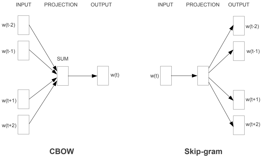
3.1 CBOW

3.1.1 Simple CBOW Model

To better understand the principles deep within the model, we will start with the Simple CBOW model (which takes one word as input and outputs one word).

As shown in the diagram above:

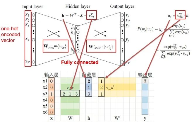
• The input layer X is the one-hot representation of the word (consider a vocabulary where each word has a number, then the one-hot representation of word W is a vector of dimension V, where the nth element is non-zero, and all other elements are zero, for example: W);
• There is a weight matrix between the input layer and the hidden layer, and the value obtained at the hidden layer is derived from multiplying the input by the weight matrix (careful readers will notice that multiplying a vector by a matrix is equivalent to selecting a certain row of the weight matrix, as shown in the figure: the input vector is W, and transposing W means selecting the nth row from the matrix as the value of the hidden layer);
• There is also a weight matrix from the hidden layer to the output layer, so each value in the output layer vector is actually the dot product of the hidden layer vector and each column of the weight vector. For example, the first number in the output layer is the result of the dot product of the vector and the column vector corresponding to the first output;
• The final output requires passing through the softmax function, which normalizes each element in the output vector to a probability between 0 and 1; the highest probability is the predicted word.

After understanding the framework of the Simple CBOW model, we will learn about its objective function.

The output layer is normalized through softmax, representing the original results of the output layer. Through the following formula, our objective function can be transformed into this form:

3.1.2 CBOW Multi-Word Context Model

After understanding the Simple CBOW model, it is easy to extend to CBOW by simply changing the single input to multiple inputs (the red line part).

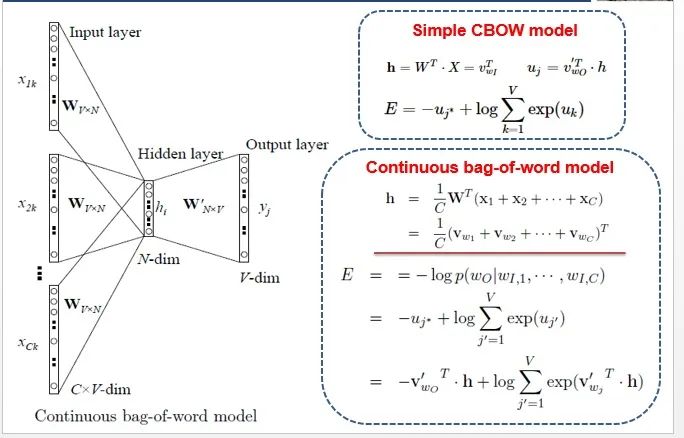
Comparing, it can be found that the difference from the simple CBOW is that the input has changed from one word to multiple words, and each input W_i reaches the hidden layer through the same weight matrix; the hidden layer values become the average of multiple words multiplied by the weight matrix.

3.2 Skip-gram Model

With the introduction of CBOW, understanding the Skip-gram model should be quicker.

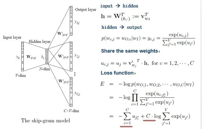
As shown in the diagram above, the Skip-gram model predicts the probabilities of multiple words by inputting one word. The principle from the input layer to the hidden layer is the same as that of the simple CBOW; the difference lies in the output layer, where the loss function becomes the total loss function for multiple words, and the weight matrix is still shared.

Generally speaking, neural network language models output the predicted probabilities of the target word, which means that every prediction requires calculations based on the entire dataset, which undoubtedly incurs a significant time cost. Unlike other neural networks, Word2Vec proposes two methods to speed up training: Hierarchical softmax and Negative Sampling.

4. Hierarchical Softmax-Based Model

The Hierarchical Softmax-based model primarily consists of an input layer, a projection layer (hidden layer), and an output layer, very similar to the neural network structure. For the CBOW model based on Hierarchical Softmax in Word2Vec, the final objective function to optimize is:

Where W represents the context words of word W. The final objective function to optimize for the Skip-gram model based on Hierarchical Softmax is:

4.1 CBOW Based on Hierarchical Softmax

4.1.1 CBOW Model Network Structure

The diagram below shows the overall structure of CBOW based on Hierarchical Softmax. First, it includes an input layer, a projection layer, and an output layer:

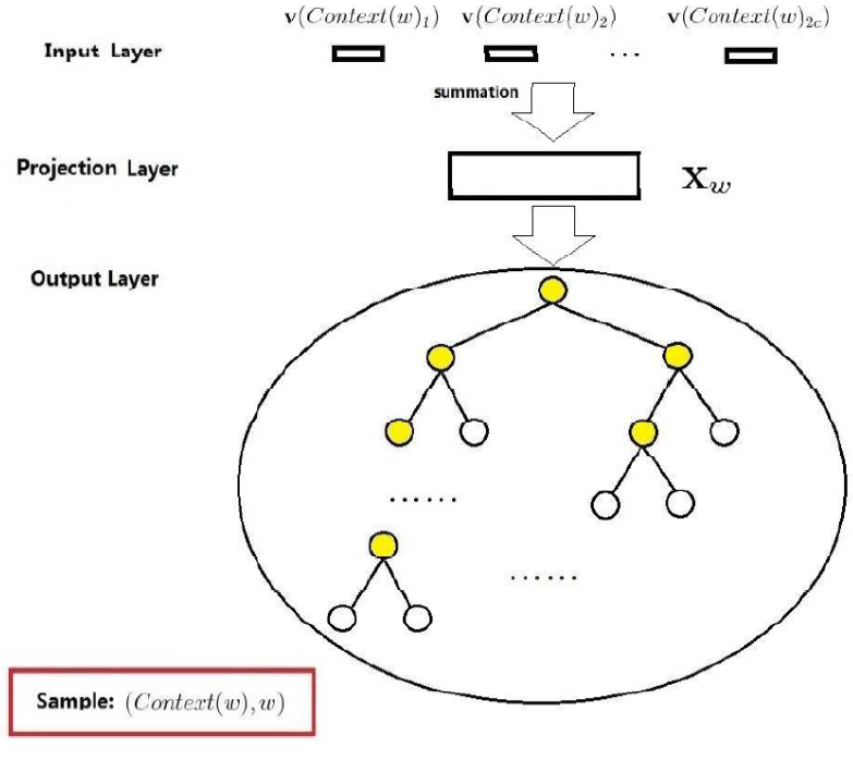
• The input layer refers to the word vectors of the W context words contained in W.
• The projection layer refers to directly summing the W word vectors, resulting in the following:

• The output layer is a Huffman tree, where the leaf nodes correspond to W words, and the non-leaf nodes correspond to the nodes marked in yellow in the above diagram. The essence of Word2Vec’s approach based on Hierarchical Softmax is concentrated in the Huffman tree part, which will be detailed below.

4.1.2 Objective Function of CBOW

To facilitate the introduction and derivation of formulas below, we need to pre-define some variables:

• Path: The path from the root node to the leaf node corresponding to word W.
• Number of Nodes: The number of nodes in path P.
• Nodes: The nodes corresponding to path P, where P represents the root node, and W represents the node corresponding to the word.
• Huffman Code: The Huffman code corresponding to word W, which consists of k bits, where b_i represents the Huffman code corresponding to the i-th node in path P, and the root node does not participate in the corresponding encoding.
• Non-leaf Node Vectors: The vectors corresponding to the non-leaf nodes in path P, representing the vectors corresponding to the i-th non-leaf node in path P. The reason for defining word vectors for non-leaf nodes is that these vectors will serve as auxiliary variables in the calculations for deriving formulas.

Now that we have introduced so many symbols, let’s use a simple example to illustrate them. We consider the case where the word w = “football.” The red line in the diagram below is the path taken by our word, and the nodes on the entire path constitute path P, with a length of k, and then the nodes on path P correspond to the five nodes, where P corresponds to the root node. The Huffman code corresponding to “football” is also shown. Finally, the vectors corresponding to the non-leaf nodes on path P are:

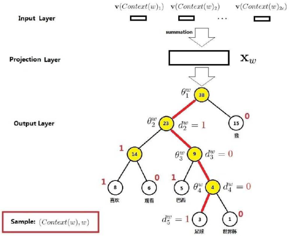
Next, we need to consider how to construct the conditional probability function P(W | context). Taking w = “football” as an example, the path from the root node to the word “football” involves k branches, that is, the red line. For this Huffman tree, each branch corresponds to a binary classification.

Since it is a binary classification, we can define one as the positive class and one as the negative class. The Huffman code for “football” is b = (0, 1, 1, 0), and the Huffman code does not include the root node because it cannot be classified as left or right subtree. Based on the Huffman code, we generally consider the positive class as the nodes in the Huffman code, while the negative class as those not in the Huffman code. However, this is just a convention, as there is no explicit requirement for the correspondence between the Huffman code and the positive and negative classes. In fact, Word2Vec defines the nodes corresponding to the Huffman code as negative classes, while those not corresponding to the Huffman code as positive classes. In other words, if classified into the left subtree, it is a negative class; if classified into the right subtree, it is a positive class. So we can define the formulas for the positive and negative classes:

In short, when classifying a node, if it goes to the left, it is a negative class; if it goes to the right, it is a positive class.

When performing binary classification, we choose the Sigmoid function. Thus, the probability of a node being classified as positive is:

And the probability of being classified as negative is P(N). Note that the formula contains V, which is the vector corresponding to the non-leaf node.

For the four binary classifications experienced from the root node to reach the leaf node “football,” we can write out the probabilities for each classification as:

• First classification: P(positive class 1)
• Second classification: P(positive class 2)
• Third classification: P(positive class 3)
• Fourth classification: P(positive class 4)

However, we are looking for P(W | context), which is the relationship between this probability value and the probability of the word “football.” The relationship is:

Thus, the basic idea of Hierarchical Softmax has been introduced through the example of w = “football.” In summary, for any word W in the vocabulary, there is a unique path from the root node to the leaf node corresponding to W, and this path exists k branches, treating each branch as a binary classification, and the probabilities generated by each classification, when multiplied together, yield the required P(W | context).

The general formula for conditional probability P(W | context) can be written as:

Where:

Or expressed as an overall expression:

Substituting formula (8) into formula (6) yields:

For ease of gradient derivation, we can simplify the double summation notation as:

Thus, we have derived the objective function formula for the CBOW model (formula 9), and the next step is to discuss how to optimize it, that is, how to maximize this function. In Word2Vec, the method used is stochastic gradient ascent. A key aspect of gradient-based algorithms is providing the corresponding gradient calculation formulas for backpropagation.

4.1.3 Parameter Update

First, consider the gradient calculation for V:

Thus, the update formula for V can be written as:

Next, consider the gradient with respect to the non-leaf node vector:

At this point, we have obtained the gradient for V, but what we actually want is the gradient for each word in the vocabulary, and V is the cumulative result for all words in the vocabulary. So how do we use V to update each word in the vocabulary? The original authors chose a straightforward approach, directly using the gradient of V to update each word in the vocabulary:

4.2 Skip-gram Based on Hierarchical Softmax

This section introduces another model in Word2Vec – the Skip-gram model. Since the derivation process is similar to that of CBOW, we will start with the objective function and use the previous notation.

4.2.1 Skip-gram Model Network Structure

The diagram below shows the network structure of the Skip-gram model. Like the CBOW model, it also consists of three layers: input layer, projection layer, and output layer. Taking the sample w as an example, we will briefly explain these three layers.

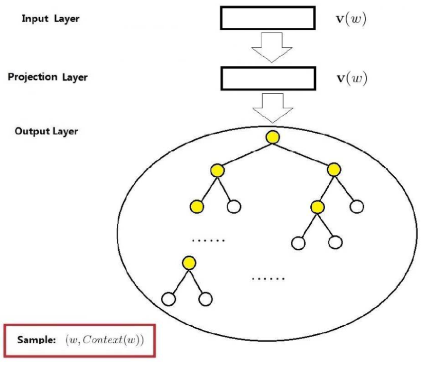
• The input layer contains only the word vector of the current sample word W.
• The projection layer performs identity projection, projecting W to itself. Hence, this projection layer is actually redundant; it is retained here mainly for comparison with the network structure of the CBOW model.
• The output layer, like the CBOW model, is also a Huffman tree.

4.2.2 Objective Function of Skip-gram

For the Skip-gram model, the known input is the current word W, and we need to predict the words in its context W_context. Therefore, the objective function should take the form of:

Where:

Or expressed as an overall expression:

Here, W_context represents the negative sample subset generated when processing word W. Thus, for a given corpus, the function:

Can serve as the overall optimization objective. Again, for ease of derivation, we take the logarithm, leading to the final objective function:

For the convenience of gradient derivation, we still extract the content under the triple summation symbol and denote it as:

Next, we will use stochastic gradient ascent to derive the gradient. First, consider the gradient with respect to V:

Then the update formula for V can be written as:

Similarly, due to symmetry, we can easily obtain the gradient for the non-leaf node vector:

Thus, the update formula for the non-leaf node vector can be written as:

5. Model Based on Negative Sampling

This section will introduce the CBOW and Skip-gram models based on Negative Sampling. Negative Sampling (abbreviated as NEG) was proposed by Tomas Mikolov et al. in the paper “Distributed Representations of Words and Phrases and their Compositionality.” It is a simplified version of NCE (Noise Contrastive Estimation) aimed at improving training speed and enhancing the quality of the resulting word vectors. Compared to Hierarchical Softmax, NEG does not use the complex Huffman tree but instead employs relatively simple random negative sampling, significantly improving performance, thus serving as an alternative to Hierarchical Softmax.

The details of NCE are somewhat complex; its essence is to use a known probability density function to estimate an unknown probability density function. In simple terms, if the unknown probability density function is X and the known probability density function is Y, once the relationship between X and Y is obtained, X can be computed. For specifics, refer to the paper “Noise-contrastive estimation of unnormalized statistical models, with applications to natural image statistics.”

5.1 Brief Introduction to Negative Sampling Algorithm

As the name implies, negative sampling is a crucial part of the CBOW and Skip-gram models based on Negative Sampling. How to generate negative samples for a given word?

Words in the vocabulary appear with varying frequencies in the corpus; for high-frequency words, the probability of being selected as negative samples should be relatively large, while for low-frequency words, the probability should be relatively small. This is a broad requirement for the sampling process, essentially a weighted sampling problem.

First, let’s use a brief description to help readers understand the mechanism of weighted sampling. Let each word in the vocabulary correspond to a line segment of length:

Here, f represents the number of times a word appears in the corpus (the summation term in the denominator is used for normalization). Now, connect these line segments end to end to form a unit line segment. If we randomly place points on this unit line segment, the longer segments (corresponding to high-frequency words) will have a higher probability of being hit.

Next, let’s discuss the specific approach in Word2Vec. Let V_i represent the i-th word in the vocabulary, and by taking V_i as the splitting point, we can obtain a non-uniform subdivision of the interval [0, 1], with k being the number of splitting intervals. We further introduce a uniform subdivision over the interval [0, 1], with splitting points being {p_j}, where j = 1, 2, …, k, as shown in the diagram below.

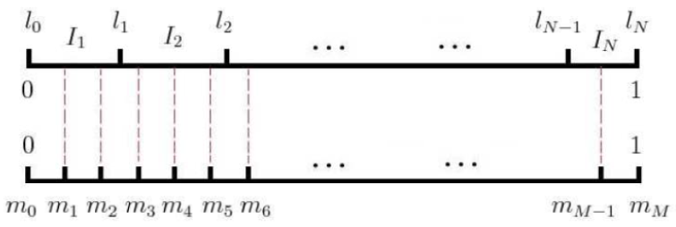
Figure: Illustration of the Mapping Establishment

With this mapping established, sampling becomes simple: each time we generate a random integer between 1 and k, that is a sample. Of course, there is one detail: when sampling for W, if we happen to select W itself, what do we do? We simply skip it; this is how Word2Vec’s code handles it.

It is worth mentioning that when setting weights for words in the vocabulary in Word2Vec’s source code, it does not directly use the frequency but raises it to the power of 0.75, making the formula:

Additionally, in the code, a variable is used to represent the exponent. The mapping formula is completed through a function called InitUnigramTable.

5.2 CBOW Based on Negative Sampling

Having introduced the negative sampling algorithm, we will now derive the objective function for CBOW based on Negative Sampling. First, we select a negative sample subset S for W. For W, we define the label of word W as:

This formula represents the label of word W, where the label of the positive sample is 1, and the label of the negative sample is 0.

For a given positive sample W, the objective function we wish to maximize is:

Where:

Here, W_context represents the sum of the word vectors in S, and V is an auxiliary vector that serves as a parameter to be trained.

Why do we want to maximize this function? Let’s take a look at the expression; substituting formula (15) into formula (14) gives:

Where P(W | context) indicates the predicted probability of the center word being W given the context, while P(W|~context) indicates the predicted probability of the center word being W given the negative context. This resembles a binary classification problem. Formally, maximizing P(W | context) corresponds to maximizing P(W) while simultaneously minimizing P(W|~context). Isn’t this what we want? To increase the probability of the positive sample while reducing the probability of the negative samples. Thus, for a given corpus, the function:

Can serve as the overall optimization objective. Of course, for the sake of derivation convenience, we take the logarithm, leading to the final objective function:

Similarly, for convenience in derivation, we take:

Next, we will use stochastic gradient ascent to derive the gradient. First, consider the gradient with respect to V:

Then the update formula for V can be written as:

Similarly, based on symmetry, we can derive the gradient for V:

The update formula for V can be written as:

5.3 Skip-gram Based on Negative Sampling

This section introduces the Skip-gram model based on Negative Sampling. Its approach is the same as that of the CBOW model introduced in the previous section, so we will start with the objective function and use the previous notation.

For a given sample W, we wish to maximize:

Where:

Or expressed as an overall expression:

Here, W_context represents the negative sample subset generated when processing word W. Thus, for a given corpus, the function:

Can serve as the overall optimization objective. Again, for ease of derivation, we take the logarithm, leading to the final objective function:

For the convenience of gradient derivation, we still extract the content under the triple summation symbol and denote it as:

Next, we will use stochastic gradient ascent to derive the gradient. First, consider the gradient with respect to V:

Then the update formula for V can be written as:

Similarly, based on symmetry, we can derive:

The update formula for V can be written as:

6. Thoughts on Several Issues Regarding Word2Vec

(1) What are the principles of the two algorithm models of Word2Vec, and how to draw the network structure?

(2) What are the network inputs and outputs? What is the activation function of the hidden layer? What is the activation function of the output layer?

(3) What is the objective/loss function?

(4) How does Word2Vec obtain word vectors?

(5) Derive how the parameters of Word2Vec are updated.

(6) Which model of Word2Vec performs better and which is faster? Why?

(7) What methods are there to accelerate training in Word2Vec?

(8) Introduce Negative Sampling; what is its impact on low-frequency and high-frequency words? Why?

(9) What are the differences and connections between Word2Vec and Latent Dirichlet Allocation (LDA)?

The above questions can be answered through this article and referenced articles, so they will not be answered in detail here.

(10) Introduce the calculation process of Hierarchical Softmax; how to incorporate Huffman into the network? How are the parameters updated? What is the impact on low-frequency and high-frequency words? Why?

Hierarchical Softmax utilizes the Huffman tree to build the tree based on word frequency, where high-frequency nodes are closer to the root node, and low-frequency nodes are farther from the root node. The farther the distance, the more parameters there are, allowing the parameters on the paths of low-frequency words to receive more training, thus yielding better results.

(11) What parameters does Word2Vec have, and are there any tuning suggestions?

• Skip-Gram is slightly slower than CBOW; it performs better on low frequencies in small datasets;
• Sub-Sampling Frequent Words can simultaneously improve algorithm speed and accuracy; sample values are suggested to be around 0.001;
• Hierarchical Softmax is more friendly to low-frequency words;
• Negative Sampling is more friendly to high-frequency words;
• The dimensionality of vectors is generally better the higher it is, but not absolute;
• Window Size: Skip-Gram is generally around 10, while CBOW is around 5.

(12) What limitations does Word2Vec have?

As a simple and easy-to-use algorithm, Word2Vec also has many limitations:

• Word2Vec only considers contextual information while ignoring global information;
• Word2Vec only considers the co-occurrence of contexts while ignoring the order of words.

7. Applications of Word2Vec in Industry

The main principle of Word2Vec is to predict words based on context, as the meaning of a word can often be derived from the sentences around it.

User behavior is also a similar time series that can be inferred through context. When users browse and interact with content, we can infer the abstract features of their behavior from their interactions, allowing us to apply word vector models to recommendation and advertising fields.

7.1 NLP Field

• Word2Vec learns word vectors that represent the semantics of words, which can be used for classification, clustering, and calculating word similarity.
• The vectors generated by Word2Vec can be directly used as input for deep neural networks to perform tasks such as sentiment analysis.

7.2 Graph Embedding

There are many Graph Embedding methods based on Word2Vec, and for specifics, refer to the paper: DeepWalk (a classic graph embedding algorithm that introduces the concepts of Word2Vec), node2vec, struc2vec, etc.

7.3 Recommendation Field

• Airbnb proposed in the paper “Real-time Personalization using Embeddings for Search Ranking at Airbnb” to compose a list of user browsing behaviors and learn item vectors using Word2Vec, which improved the click-through rate by 21% and drove 99% of booking conversion rates. This paper mainly made improvements based on the Skip-gram model.

• Yahoo proposed in the paper “E-commerce in Your Inbox: Product Recommendations at Scale” to extract products from shopping receipts sent to users and compose a list, using Word2Vec to learn and recommend potential products;

7.4 Advertising Field

Yahoo proposed in the paper “Scalable Semantic Matching of Queries to Ads in Sponsored Search Advertising” to compose a list of user search queries and ads and learn feature vectors for them, enabling suitable ads to be matched for a given search query.

8. References

[1] Rong X. word2vec parameter learning explained[J]. arXiv preprint arXiv:1411.2738, 2014.[2][Paper] Word2Vec: A Silver Bullet for Word Embedding, link: https://mp.weixin.qq.com/s/7dsjfcOfm9uPheJrmB0Ghw[3] Detailed Explanation of Word2Vec – Formula Derivation and Code – link-web article – Zhihu https://zhuanlan.zhihu.com/p/86445394[4] The Illustrated Word2vec, Jay Alammar, link: https://jalammar.github.io/illustrated-word2vec/[5] Visual Explanation of Word2vec (Original Translation), link: https://mp.weixin.qq.com/s/Yq_-1eS9UuiUBhNNAIxC-Q[6] What advantages does word2vec have over previous Word Embedding methods? – Zhihu https://www.zhihu.com/question/53011711[7] [NLP] Understand the essence of word vectors Word2vec in seconds – Mu Wen’s article – Zhihu https://zhuanlan.zhihu.com/p/26306795[8] http://mccormickml.com/2016/04/19/word2vec-tutorial-the-skip-gram-model/[9] In-depth analysis of the word2vec model – TianMin’s article – Zhihu https://zhuanlan.zhihu.com/p/85998950[10] A Neural Probabilistic Language Model – Zhang Jun’s article – Zhihu https://zhuanlan.zhihu.com/p/21240807[11] What applications does word2vec have? – Zhihu https://www.zhihu.com/question/25269336

Finally, in addition to the cited references, some materials I have read are also recommended: [1] “Deep Learning Word2vec Learning Notes”, North Wandering Son. [2] “Mathematics in Word2Vec”, peghoty. [3] “Practical Word2Vec in Deep Learning”, NetEase Youdao.

Important! The WeChat academic exchange group for Natural Language Processing has been established.

You can scan the QR code below to join the group for discussion.

Note: Please modify the remarks when adding as [School/Company + Name + Direction]

For example – Harbin Institute of Technology + Zhang San + Dialogue System.

Account owner, please avoid being a micro-business. Thank you!

Recommended Reading: [Long Article Explanation] From Transformer to BERT Model<br/>Saier Translation | Understanding Transformer from Scratch<br/>A picture is worth a thousand words! A step-by-step guide to building a Transformer with Python