“ This article provides a detailed explanation of the two structures in word2vec: CBOW and skip-gram, as well as the two optimization techniques: hierarchical softmax and negative sampling. Understanding these details and principles of the word2vec algorithm is very helpful!”
Source: TianMin https://zhuanlan.zhihu.com/p/85998950
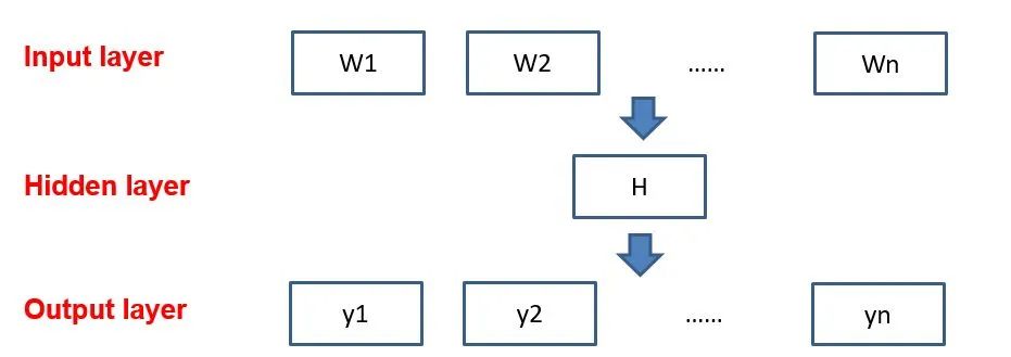
Word2vec is a lightweight neural network model that consists of an input layer, a hidden layer, and an output layer. Depending on the input and output, the model framework mainly includes CBOW and skip-gram models. The CBOW model predicts the target word based on the context, while the skip-gram does the opposite, predicting the context words based on the target word. By maximizing the probability of word occurrences, we train the model to obtain the weight matrix between the layers. The word embedding vector we refer to is derived from this weight matrix.
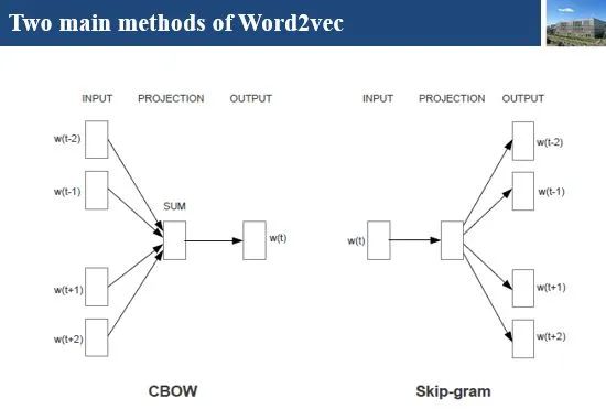
1. CBOW
(1) Simple CBOW Model
To better understand the underlying principles of the model, we will start with the Simple CBOW model (inputting one word and outputting one word) framework.
As shown in the figure:
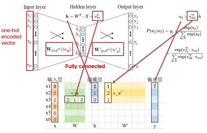
a. The input layer input X is the one-hot representation of a word (consider a vocabulary V, where each word wi has an index i∈1,…,. The one-hot representation of word wi is a vector of dimension |V|, where the i-th element is non-zero, and all other elements are zero, for example: w2=[0,1,0,…,0]T);
b. There is a weight matrix W between the input layer and the hidden layer. The value obtained at the hidden layer is derived from input X multiplied by the weight matrix (careful observers will notice that multiplying a 0-1 vector by a matrix effectively selects a particular row from the weight matrix. For instance, if the input vector X is [0,0,1,0,0,0], multiplying the transpose of W by X selects the third row [2,1,3] as the value for the hidden layer);
c. There is also a weight matrix W’ from the hidden layer to the output layer. Thus, each value in the output layer vector y is actually the dot product of the hidden layer vector with each column of the weight vector W’. For example, the first number in the output layer, 7, is the result of the dot product of vector [2,1,3] and column vector [1,2,1].
d. The final output needs to pass through the softmax function (if you don’t understand, you can search for it), which normalizes each element in the output vector to a probability between 0 and 1, with the highest probability being the predicted word.
After understanding the framework of the Simple CBOW model, let’s learn about its objective function.
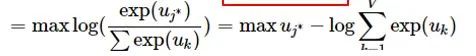
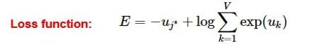
The training method is the classic backpropagation and gradient descent (not the focus of this chapter, so we won’t elaborate).
(2) CBOW
Once we understand the Simple CBOW model, extending it to CBOW is straightforward, as it simply replaces single input with multiple inputs (highlighted in red).
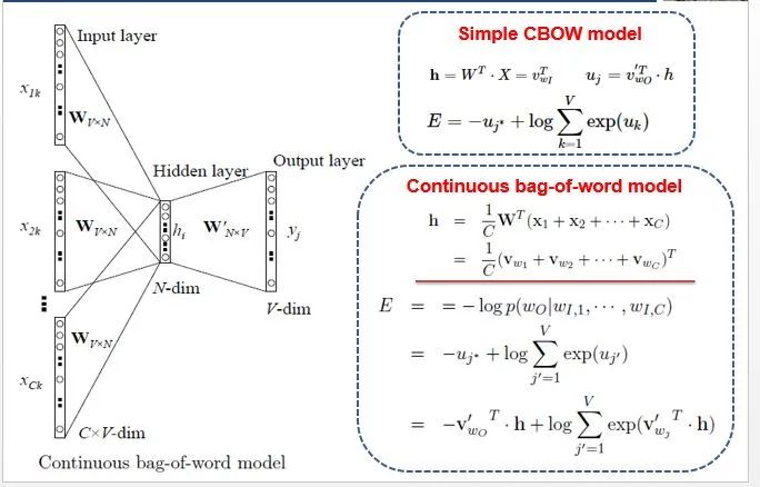
Comparing the two, we can see that unlike the simple CBOW, the input changes from 1 to C, where each input Xik reaches the hidden layer through the same weight matrix W, and the value of the hidden layer h becomes the average of multiple words multiplied by the weight matrix.
2. Skip-Gram Model
With the introduction of CBOW, understanding the skip-gram model should be quicker.
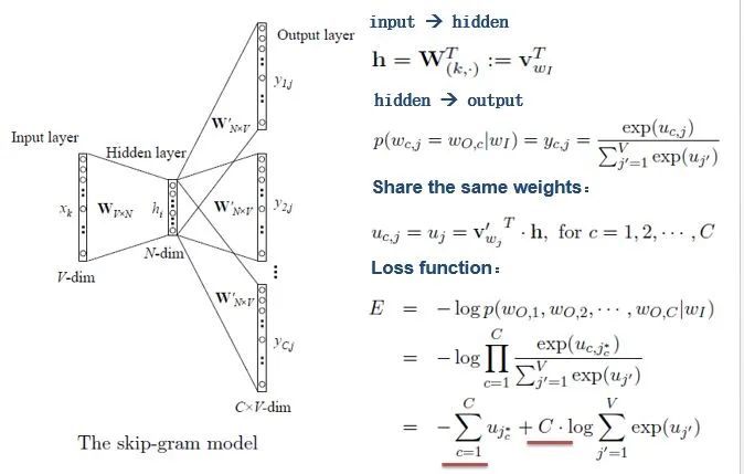
As shown in the figure:
The skip-gram model predicts the probabilities of multiple words based on a single input word. The principle from the input layer to the hidden layer is the same as that of the simple CBOW, but the difference lies in the output layer, where the loss function becomes the sum of the loss functions for C words, and the weight matrix W’ is still shared.
3. Word2Vec Model Training Mechanism (Optimization Methods)
Generally, neural network language models predict the probability of the target word, meaning that each prediction requires calculations based on the entire dataset, which undoubtedly results in a significant time overhead. Unlike other neural networks, word2vec proposes two methods to speed up training: Hierarchical softmax and Negative Sampling.
(1) Hierarchical Softmax
Prerequisite knowledge: Huffman coding, as shown in the figure:
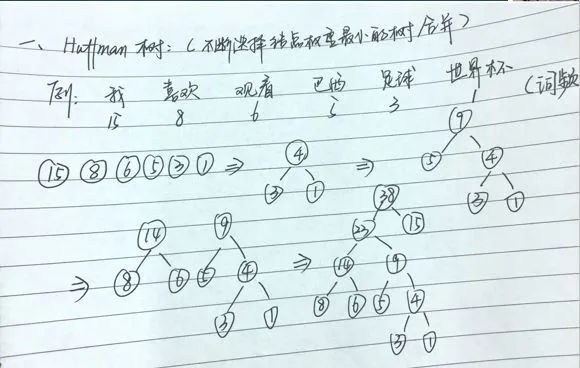
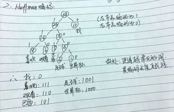
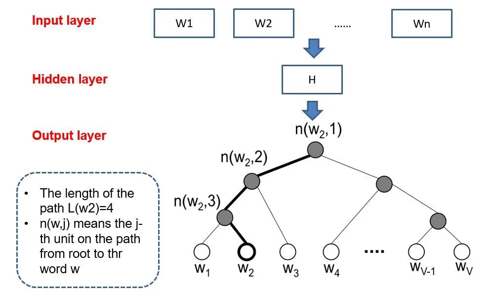
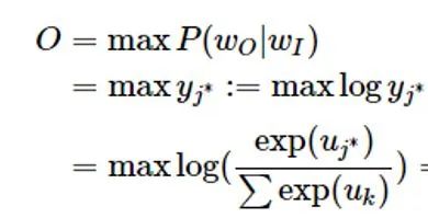
Unlike traditional neural network outputs, the hierarchical softmax structure of word2vec replaces the output layer with a Huffman tree. In the figure, the white leaf nodes represent all |V| words in the vocabulary, while the black nodes represent non-leaf nodes. Each leaf node corresponds to a unique path from the root node. Our goal is to maximize the probability of the path w=wO, i.e., P(w=wO|wI) is maximized. Assuming the final output conditional probability is W2 maximum, then I only need to update the vectors of the nodes along the path from the root to leaf node w2, rather than updating the occurrence probabilities of all words, which greatly reduces the time for model training updates.
How can we obtain the probability of a particular leaf node?
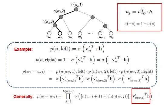
Suppose we want to calculate the probability of leaf node W2; we need to calculate the product of probabilities from the root node to the leaf node. We know that the model only replaces the softmax layer of the original model, so the value of any non-leaf node is still the result from the hidden layer to the output layer, denoted as uj. After applying sigmoid to this result, we obtain the probability p of moving to the left subtree, with 1-p being the probability of moving to the right subtree. The training method for this tree is quite complex but also involves methods such as gradient descent. For those interested, you can read the paper “word2vec Parameter Learning Explained”.
(2) Negative Sampling
In traditional neural networks, each step of the training process requires calculating the probability values of other words in the vocabulary under the current context, which results in a massive computational load.
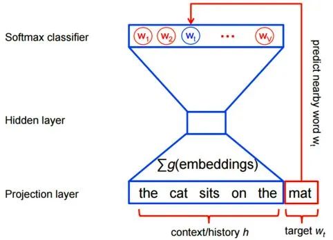
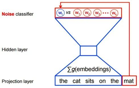
However, for feature learning in word2vec, a complete probability model is not necessary. The CBOW and Skip-Gram models use a binary classifier (i.e., Logistic Regression) at the output end to distinguish between the target word and k other words in the vocabulary (where the target word is one class and the other words are another class). Below is an illustration of a CBOW model, where the input and output for the Skip-Gram model are reversed.
At this point, the maximized objective function is as follows:
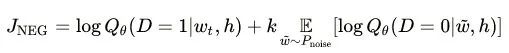
Where Qθ(D=1|w,h) is the probability of “binary logistic regression”, specifically the probability of word w appearing in dataset D given the embedding vector θ and context h. The latter part of the formula represents the expected value of the probabilities of k words randomly selected from the [noise dataset] appearing (in log form). The significance of the objective function is evident: to assign the highest probability to the actual target word while assigning low probabilities to the other k [noise words]. This technique is referred to as “Negative Sampling”.
This idea stems from the “Noise Contrastive Estimation (NCE)” method, which generally posits: Suppose X=(x1,x2,⋯,xTd) is a sample drawn from real data (or corpus), but we do not know the distribution of the samples. We assume each xi follows an unknown probability density function pd. Thus, we need a relatively referenceable distribution to estimate the probability density function pd, which can be a known distribution such as Gaussian or uniform. Suppose the probability density function of this noise distribution is pn, with samples drawn from it being Y=(y1,y2,⋯,yTn), which are termed noise samples. Our goal is to learn a classifier to distinguish between these two types of samples and learn the properties of the data from the model. The idea of noise contrastive estimation is “learning through comparison.”
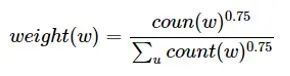
Specifically, in word2vec, negative sampling involves dividing the V samples at the output layer into positive samples (the target word) and the remaining V−1 negative samples. For example, for a sample phonenumber, wI=phone, wO=number, the positive sample is the word number, while the negative samples are words that are unlikely to co-occur with phone. The idea of negative sampling is to randomly select a small portion of negative samples during each training iteration to minimize their probabilities while maximizing the corresponding positive sample probabilities. Random sampling requires assuming a probability distribution, and in word2vec, we directly use word frequency as the distribution of words, modifying it by raising the frequency to the power of 0.75. This approach reduces the impact of large differences in frequency, increasing the probability of less frequent words being sampled.
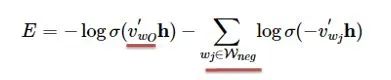
The loss function defined by negative sampling is as follows:
If you still don’t have a deep understanding, we will further enhance our understanding through the official TensorFlow word2vec code released by Google. Code link: https://github.com/tensorflow/tensorflow/blob/master/tensorflow/examples/tutorials/word2vec/word2vec_basic.py
To learn more, please scan the QR code below and follow the Machine Learning Research Society

Source: Shallow Dream’s Study Notes