In-Depth Analysis of Word2Vec Model

Source | Zhihu Author | TianMin

Link丨https://zhuanlan.zhihu.com/p/85998950

Editor | Deep Learning Matters WeChat Official Account

This article is for academic exchange only. If there is any infringement, please contact for removal.

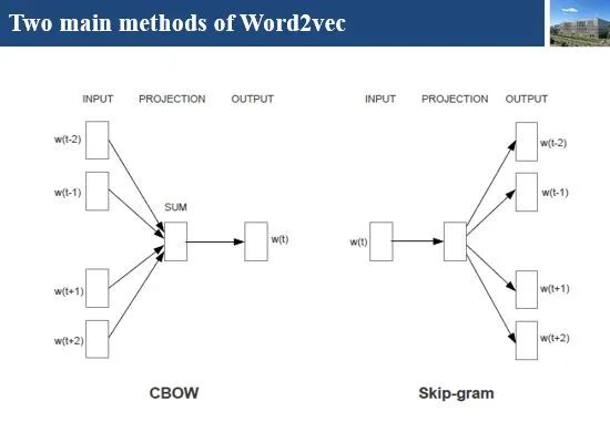
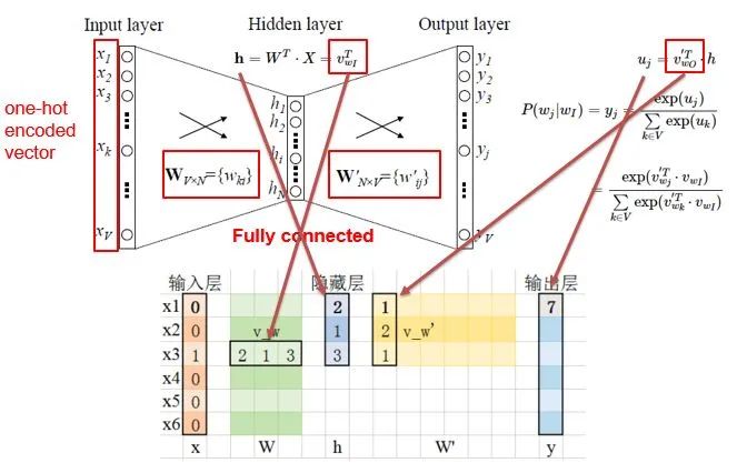
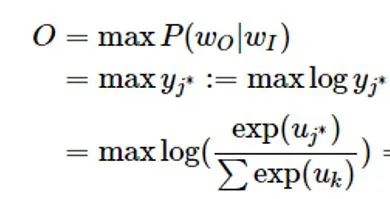
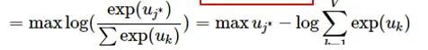
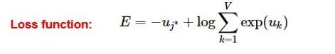
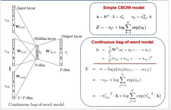
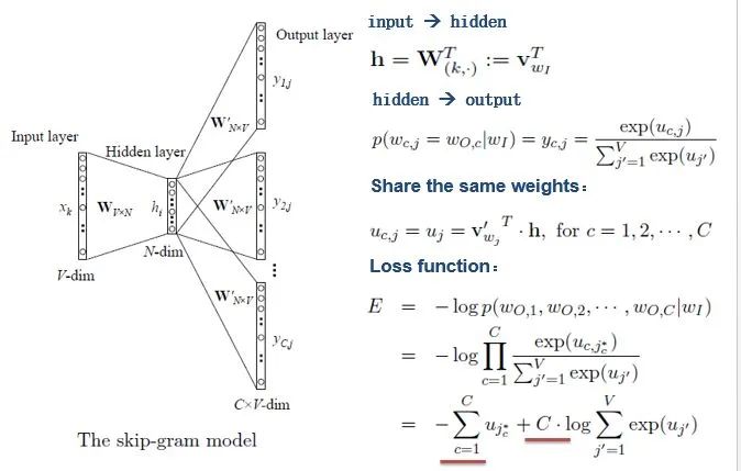
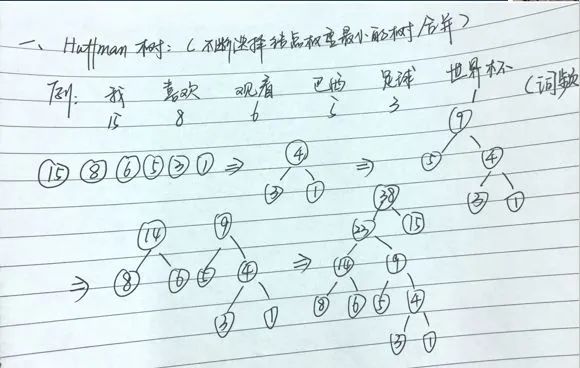
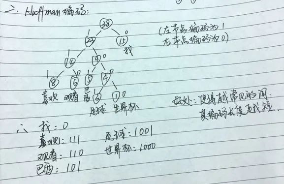
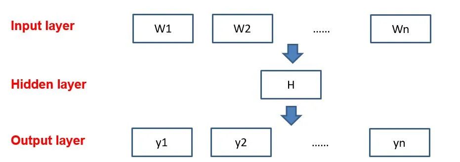
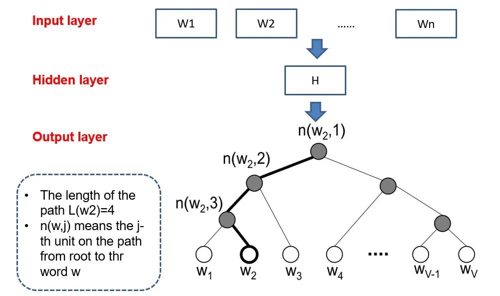
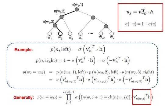
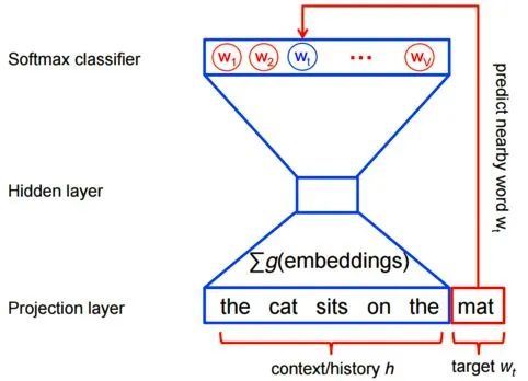
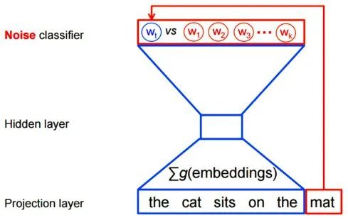
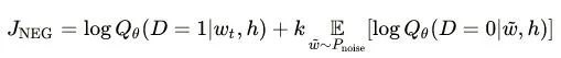
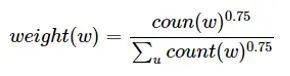
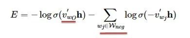
[Introduction] Word2Vec is a widely used word embedding method. Due to recent research needs, I studied the algorithm model. Since there is a lot of content about Word2Vec, I will try to explain the core content. Please point out any shortcomings!

Word2Vec is a lightweight neural network, and its model only includes an input layer, a hidden layer, and an output layer. The model framework mainly includes CBOW and skip-gram models, depending on the input and output. The CBOW model predicts the target word based on the context, while skip-gram predicts the context words based on the target word. By maximizing the probability of word occurrences, we can train the model to obtain the weight matrix between each layer. The word embedding vector we refer to is derived from this weight matrix.

1. CBOW

(1) Simple CBOW model

To better understand the principles behind the model, we will start with the Simple CBOW model (which takes one input word and outputs one word).

As shown in the figure:

a. The input layer’s X is the one-hot representation of the word (considering a vocabulary V, where each word wi has an index i∈{1,…,|V|}. The one-hot representation of word wi is a vector of dimension |V|, where the i-th element is non-zero and all other elements are zero, for example: w2=[0,1,0,…,0]T);

b. There is a weight matrix W between the input layer and the hidden layer. The value obtained at the hidden layer is derived from multiplying the input X by the weight matrix (careful readers will notice that multiplying a 0-1 vector by a matrix effectively selects a specific row from the weight matrix. For example, if the input vector X is [0, 0, 1, 0, 0, 0], multiplying the transpose of W by X selects the third row [2,1,3] as the hidden layer’s value);

c. There is also a weight matrix W’ between the hidden layer and the output layer. Therefore, each value in the output layer vector y is actually the dot product of the hidden layer vector with each column of the weight vector W’. For example, the first number of the output layer, 7, is the result of the dot product of the vector [2,1,3] and the column vector [1,2,1].

d. The final output must go through the softmax function (if you don’t understand, you can search for it). This function normalizes each element in the output vector to a probability between 0 and 1, and the one with the highest probability is the predicted word.

After understanding the framework of the Simple CBOW model, let’s learn about its objective function.

Output layer softmax, u represents the original output of the output layer

The training method is the classic backpropagation and gradient descent (this is not the focus of this chapter, so I won’t elaborate).

(2) CBOW

Once we understand the Simple CBOW model, extending it to CBOW is easy; we simply replace the single input with multiple inputs (the part marked in red).

Comparing, we can find that the difference from simple CBOW is that the input has changed from 1 to C, and each input Xik reaches the hidden layer through the same weight matrix W. The value of the hidden layer h becomes the average of multiple words multiplied by the weight matrix.

2. Skip-Gram Model

With the introduction of CBOW, understanding the skip-gram model should be quicker.

As shown in the figure:

The skip-gram model predicts the probabilities of multiple words based on a single input word. The principle from the input layer to the hidden layer is the same as in simple CBOW, but the loss function from the hidden layer to the output layer becomes the sum of the loss functions of C words, and the weight matrix W’ is still shared.

3. Word2Vec Model Training Mechanism (Optimization Methods)

Generally, neural network language models predict the probability of the target word, which means each prediction requires calculations based on the entire dataset, leading to significant time overhead. Unlike other neural networks, word2vec proposes two methods to accelerate training: Hierarchical softmax and Negative Sampling.

(1) Hierarchical Softmax

Prerequisite knowledge: Huffman coding, as shown in the figure:

Unlike the outputs of traditional neural networks, the hierarchical softmax structure of word2vec replaces the output layer with a Huffman tree. The white leaf nodes in the figure represent all |V| words in the vocabulary, while the black nodes represent non-leaf nodes. Each leaf node corresponds to a unique path from the root node. Our goal is to maximize the probability of the path w=wO, i.e., maximize P(w=wO|wI). Assuming the conditional probability output is W2, we only need to update the vector of the nodes along the path from the root to w2, rather than updating the occurrence probabilities of all words, significantly reducing the training update time.

How do we obtain the probability of a leaf node?

To calculate the probability of the leaf node W2, we need to compute the product of probabilities from the root node to the leaf node. We know that this model only replaces the softmax layer of the original model, so the value of a non-leaf node is still the result from the hidden layer to the output layer, uj. After applying sigmoid to this result, we obtain the probability p of going left in the subtree, and 1-p for going right. The training method for this tree is complex, but it also uses gradient descent and other methods. Interested readers can refer to the paper Word2Vec Parameter Learning Explained.

(2) Negative Sampling

In traditional neural networks, each step of the training process requires calculating the probabilities of other words in the vocabulary under the current context, which leads to a massive computation load.

However, for feature learning in word2vec, a complete probability model is not necessary. The CBOW and Skip-Gram models use a binary classifier (i.e., Logistic Regression) at the output to distinguish the target word from k other words in the vocabulary (i.e., treating the target word as one class and the others as another class). Below is a diagram of a CBOW model; for the Skip-Gram model, the input and output are inverted.

At this point, the maximization objective function is as follows:

Where Qθ(D=1|w,h) is the binary logistic regression probability, specifically the probability of word w appearing in dataset D given the embedding vector θ and context h; the latter part of the formula is the expected value of the log probability of k words randomly selected from the [noise dataset]. It is clear that the objective function aims to assign a high probability to the real target word and a low probability to the other k [noise words]. This technique is known as Negative Sampling.

This idea is derived from the noise contrastive estimation (NCE) method, which roughly states: assume X=(x1,x2,…,xTd) is a sample drawn from real data (or corpus), but we do not know the distribution of the samples. We assume each xi follows an unknown probability density function pd. We need a reference distribution to estimate pd, which we can know, such as Gaussian or uniform distribution. Assume the probability density function of this noise distribution is pn, from which we draw sample data Y=(y1,y2,…,yTn). Our goal is to learn a classifier to distinguish between these two types of samples and learn the properties of the data from the model; the idea of noise contrastive estimation is to “learn through comparison.”

Specifically, in word2vec’s negative sampling: we divide the V samples at the output layer into positive samples (the target word) and V−1 negative samples. For example, in the sample “phone number”, wI=phone and wO=number, the positive sample is the word number, and the negative samples are those words that are unlikely to co-occur with phone.

The idea of negative sampling is to randomly select a small number of negative samples during training to minimize their probabilities while maximizing the corresponding positive sample probabilities.

Random sampling requires assuming a probability distribution. In word2vec, the word frequency is directly used as the distribution, but with the frequency raised to the power of 0.75. This approach mitigates the impact of large differences in frequency, increasing the probability of sampling low-frequency words.

The loss function defined by negative sampling is as follows:

If you still don’t fully understand, I will analyze the official TensorFlow Word2Vec code released by Google to deepen understanding.

Code link:

https://github.com/tensorflow/tensorflow/blob/master/tensorflow/examples/tutorials/word2vec/word2vec_basic.py

I will provide a detailed analysis of the code later, so stay tuned~ Thank you

Recommended Reading: Related Papers



—The End—
Recommended for you
Top Ten Influential Female Scientists in AI
Latest Deep Learning Intro Course from MIT, Let's Get Started!
With this tool, easily write an App in Python
"The Most Comprehensive" holds true, NumPy has had an official Chinese tutorial for a long time
Comic version of the Linux Kernel World

Leave a Comment Cancel reply