

This article is translated from the blog below.
https://jalammar.github.io/illustrated-word2vec/

I think the concept of embeddings is one of the most fascinating ideas in machine learning. If you have ever used Siri, Google Assistant, Alexa, Google Translate, or even a smartphone keyboard with next-word prediction features, you have likely benefited from this idea, which has become central to natural language processing models. Over the past few decades, the application of embeddings in neural models has seen significant development (recent advancements include context-based word embeddings, leading to cutting-edge models like BERT and GPT2).
Word2Vec is an efficient method for creating word embeddings, and it has been in use since 2013. However, beyond being a method for word embeddings, some of its concepts have proven to be very effective in creating recommendation engines and understanding continuous data in non-linguistic business tasks. Companies like Airbnb, Alibaba, Spotify, and Anghami have leveraged the power of NLP to empower a new type of recommendation engine.
In this article, we will introduce the concept of embeddings and the mechanism of generating embeddings using Word2Vec. But first, let’s start with an example to understand how to represent things using vectors. Did you know that a list of five numbers (a vector) can represent a lot of information about your personality?
Personality Embeddings: What Kind of Person Are You?
On a scale from 0 to 100, how introverted/extroverted are you (where 0 is the most introverted and 100 is the most extroverted)? Have you taken personality tests like MBTI (Myers-Briggs Type Indicator) or the better-known Big Five personality traits test? If you haven’t taken one, these tests will ask you a series of questions and then score you across several dimensions, of which introversion/extroversion is one.

Let’s say I scored 38/100 on the introversion/extroversion scale. I could plot it like this:

Now, let’s narrow the range to -1 to 1:
How much do you think you understand a person based solely on this one piece of information? Not much. People are complex. So let’s add another dimension – another trait from the personality test.

We can represent the two dimensions as a point on a graph, or as a vector from the origin to that point. We have great tools to handle the upcoming vectors.
I’ve hidden the personality traits we’re plotting so you won’t know what each dimension represents, but you can still gain a lot of information from the vector representation of personality.
Now we can say this vector partially represents my personality. The usefulness of this representation comes when you want to compare two other people to me. Let’s say I get hit by a bus and need to find someone with a similar personality to replace me. In the graph below, which person is more similar to me?

A common method for calculating similarity scores when dealing with vectors is cosine similarity:

Person 1 is more similar in personality to me. Vectors pointing in the same direction (length also matters) have a higher cosine similarity.
Once again, two dimensions cannot capture enough information about the differences between people. Decades of psychological research have identified five main traits (as well as many secondary traits). So let’s use all five dimensions in our comparison:

The problem with using five dimensions is that we lose the ability to neatly plot little arrows in two-dimensional space. This is a common challenge in machine learning, where we often need to think in higher-dimensional spaces. The good news is that cosine similarity still applies. It works for any number of dimensions:

Cosine similarity works for any number of dimensions. These scores are better than the last ones because they are calculated based on higher-dimensional comparisons.
At the end of this section, I would like to present two central ideas:
1. We can represent people and things as algebraic vectors (which is great for machines!).
2. We can easily calculate the relationships between similar vectors.

Word Embeddings
With this understanding, we can continue to look at examples of trained word vectors (also known as word embeddings) and start exploring some of their interesting properties.
Here is the word embedding for the word “king” (trained GloVe vectors from Wikipedia):
[ 0.50451 , 0.68607 , -0.59517 , -0.022801, 0.60046 , -0.13498 , -0.08813 , 0.47377 , -0.61798 , -0.31012 , -0.076666, 1.493 , -0.034189, -0.98173 , 0.68229 , 0.81722 , -0.51874 , -0.31503 , -0.55809 , 0.66421 , 0.1961 , -0.13495 , -0.11476 , -0.30344 , 0.41177 , -2.223 , -1.0756 , -1.0783 , -0.34354 , 0.33505 , 1.9927 , -0.04234 , -0.64319 , 0.71125 , 0.49159 , 0.16754 , 0.34344 , -0.25663 , -0.8523 , 0.1661 , 0.40102 , 1.1685 , -1.0137 , -0.21585 , -0.15155 , 0.78321 , -0.91241 , -1.6106 , -0.64426 , -0.51042 ]
You can try this out using the online tool below.
WebVectors: An interactive word vector playground for NLP
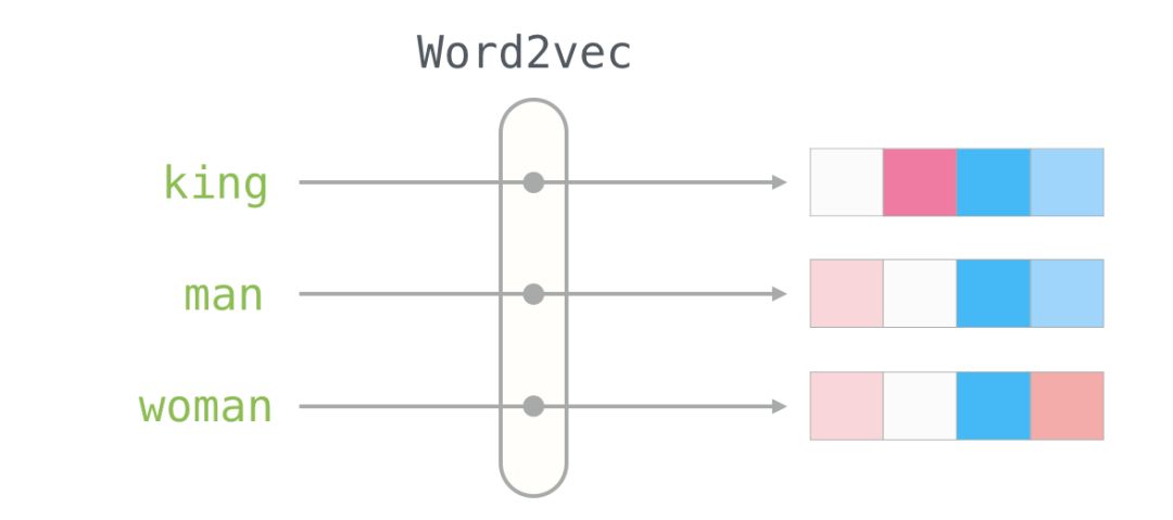
This is a list of 50 numbers. By looking at these values, we can’t derive much information. But let’s visualize it a bit to compare it with other word vectors. Let’s put all these numbers in a row:

Let’s color the cells based on the size of the values (red if close to 2; white if close to 0; blue if close to -2):

We will ignore the numbers and focus on the colors to represent the values of the cells. Now let’s compare “King” with other words:

You can see that “Man” and “Woman” are more similar to each other than either is to “King.” This tells you something. These vector representations capture a lot of information, meanings, and associations about these words.
This is another example list (by vertically scanning the columns, looking for color-similar columns to compare):

Notice a few things:
1. Among all these different words, there is one column that is red. They are similar in this dimension (and we don’t know what each dimension represents). 2. You can see that “woman” and “girl” are similar in many places. Similarly, “man” and “boy” are as well. 3. “boy” and “girl” also have some places where they are similar to each other but differ from “woman” or “man.” Could this represent a vague concept of “youth”? Possibly. 4. Except for the last word, all the words represent people. I added an object (“water”) to show the differences between categories. For example, you can see that the blue column extends all the way down and then stops before the embedding for “water.” 5. There are clear places where “king” and “queen” are similar to each other and different from all other words. Could these represent a vague concept of “royalty”?
Analogies
A famous example showcasing the wonderful properties of embeddings is analogies. We can add and subtract word embeddings and get interesting results. One famous example is the formula: “king” – “man” + “woman”:

Using the Gensim library in Python, we can add and subtract word vectors, and it will find the words most similar to the resulting vector. This image shows the list of most similar words, each with its cosine similarity.
We can visualize this analogy as before:

The vector generated from “king – man + woman” isn’t exactly equal to “queen,” but “queen” is the closest word to it among the 400,000 word embeddings we have here.
Now that we have seen trained word embeddings, let’s learn more about the training process. But before we start with Word2Vec, we need to look at the parent concept of word embeddings: language models.
Language Models
If I had to give the most typical example of natural language processing, it would be the next-word prediction feature in smartphone input methods. This is a feature used hundreds of times a day by billions of people.

Next-word prediction is a task that can be accomplished through language models. A language model tries to predict the next word based on a list of words (say, two words) that come before it.
In the screenshot above, we can think of the model receiving two green words (thou shalt) and recommending a set of words (“not” is one of the most likely to be selected):
We can imagine this model as a black box:

But in fact, the model doesn’t just output one word. It actually scores all the words it knows (the model’s vocabulary, which could be thousands to millions of words) by probability, and the input method program selects the highest-scoring word to recommend to the user.

The output of a natural language model is the probability scores of the words the model knows, which we usually express as percentages, but in reality, a score like 40% is represented as 0.4 in the output vector set.
Natural language models (see Bengio 2003) complete predictions in three steps after training:
The first step is the most relevant to us because we are discussing Embedding. After training, the model generates a mapping matrix for all the words in its vocabulary. During prediction, our algorithm queries the input words in this mapping matrix and calculates the predicted values:
Now let’s focus on model training to learn how to construct this mapping matrix.
Language Model Training
Language models have a huge advantage over most other machine learning models. This advantage lies in the fact that we can train them using a massive amount of running text. Imagine all the books, articles, Wikipedia content, and other forms of text data we have. This is a big contrast compared to many other machine learning models that require handcrafted features and special data collection.
We can obtain their mapping relationships by finding words that frequently appear near each other. The mechanism is as follows:
1. First, obtain a large amount of text data (e.g., all Wikipedia content)
2. Then we establish a sliding window that can glide along the text (for example, a window containing three words)
3. Using this sliding window, we can generate a large amount of sample data for training the model.
As this sliding window glides over the text, we (virtually) generate a dataset for training the model. To understand how this is accomplished, let’s see how the sliding window handles this phrase:
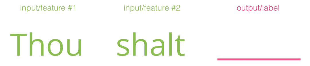
At the beginning, the window locks on the first three words of the sentence:
We take the first two words as features, and the third word as the label:
This produces the first sample in the dataset, which will be used in our subsequent language model training.
Next, we slide the window to the next position and produce the second sample:
Now the second sample is generated.
Before long, we can obtain a large dataset, from which we can see the words that tend to follow different groups of words:
In fact, the model training often occurs simultaneously while the sliding window is moving. But logically, it is clearer to separate the “dataset generation” phase from the training phase. Besides neural network-based language modeling methods, a technique called N-gram is often used for training language models (see Chapter 3 of “Speech and Language Processing”). To understand how the transition from N-gram to neural models is reflected in real-world products, here’s a blog post from 2015 by my favorite Android keyboard Swiftkey, detailing their neural language model and comparing it with the previous N-gram model. I love this example because it shows how to describe the algorithmic characteristics of embedding vectors in marketing language.
Considering Both Ends
Fill in the blanks based on the information above:
The context here is the five words before the blank (and the previously mentioned “bus”). I believe most people would guess that the blank should be filled with the word “bus.” But if I give you one more piece of information – a word after the blank – will that change your answer?
This completely changes what should fill in the blank. Now, the most likely word to fill in the blank is “red.” We can conclude that the specific words before and after a word carry information value. It turns out that considering both the left and right sides (the words on the left and right of the word we are guessing) leads to better word embeddings. Let’s see how to adjust the way we train our model to address this issue.
Skipgram Model
Instead of just looking at the two words before the target word, we can also look at the two words after it.

If we do this, the model we actually build and train looks like this:
This is called the Continuous Bag of Words structure, and it is described in a paper on Word2Vec. Another architecture has also shown good results, but it operates a bit differently.
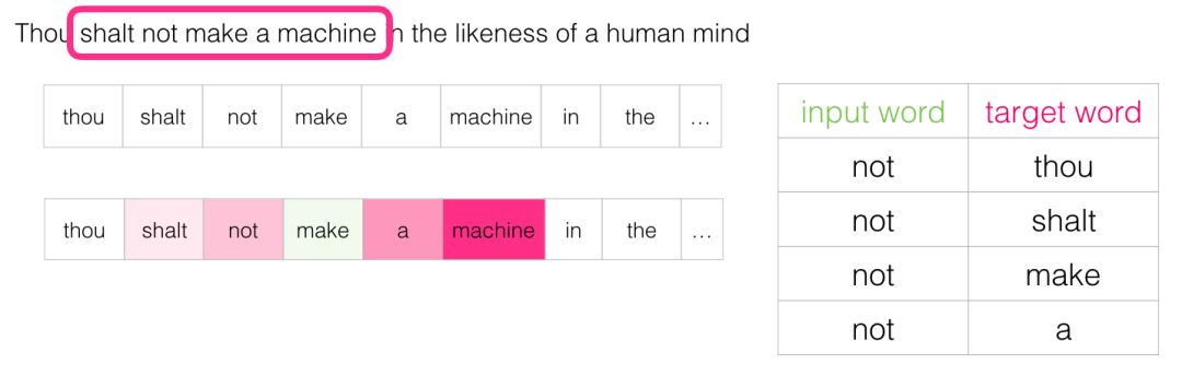
This architecture tries to guess the neighboring words using the current word instead of using the context (the words before and after) to guess the word. We can see the sliding window as follows:
The words in the green box are input words, while the pink box shows possible output results.
The depth of color in the pink box indicates the different possibilities because the sliding window generates four independent samples for the training set:
This method is called the Skipgram architecture. We can display the contents of the sliding window as follows.
This provides four samples for the dataset:
Then we move the sliding window to the next position:
Now we generate the next four samples:
After moving a few sets of positions, we can obtain a batch of samples:
Revisiting the Training Process
Now that we have the skipgram training dataset extracted from existing running text, let’s briefly look at how to use it to train a basic neural language model that can predict neighboring words.
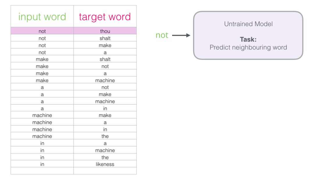
We take the first sample from the dataset. We extract features and input them into the untrained model, asking it to predict a suitable neighboring word.
The model executes these three steps and outputs a prediction vector (assigning a probability to each word in its vocabulary). Since the model is untrained, the predictions at this time are certainly incorrect. But that’s okay; we know what it should guess – the label/output unit in the row we’re currently using to train the model:
The target word probability is 1, while the probabilities for all other words are 0, so the vector composed of these values is the “target vector.”
How far off is the model’s prediction from the actual label? We subtract the two vectors to get an error vector:
Now we can use this error vector to update the model, so that next time when the model sees “not” as input, it’s more likely to guess “thou.”
This completes the first step of training. We continue the same process for the next sample in the dataset and then the next sample, until we have covered all samples in the dataset. This completes one training cycle. We can train through multiple cycles, and then we will have a trained model from which we can extract the embedding matrix for any further applications.
While this expands our understanding of the process, we still lack some key ideas about the actual training of Word2Vec.
Negative Sampleing
Recall the three steps the neural language model takes to compute prediction values:
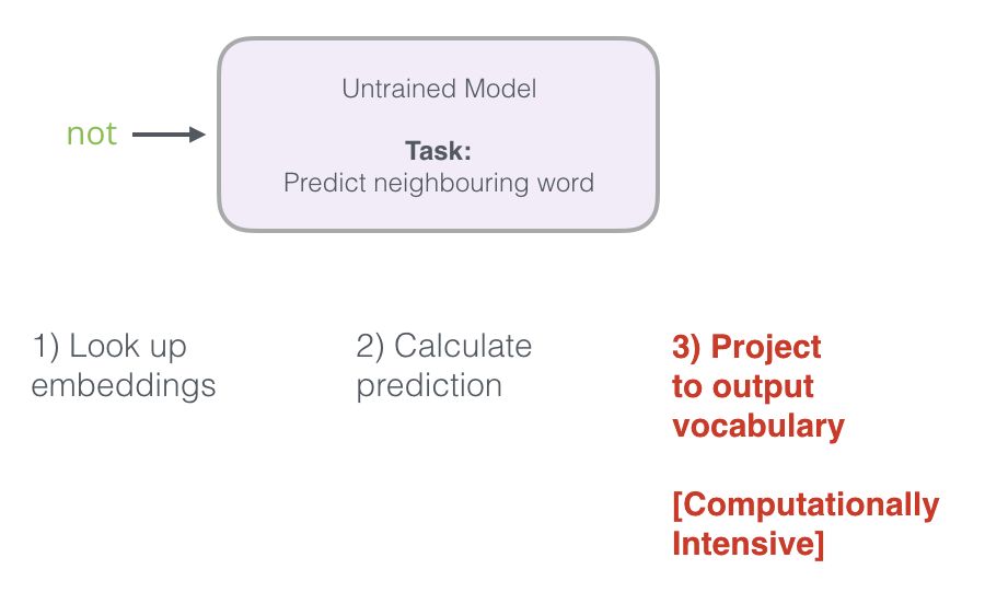
The third step is computationally expensive, especially considering that we need to perform it once for each training sample in the dataset (which can reach tens of millions). We need to take some measures to improve performance.
One approach is to divide the target into two steps:
1. Generate high-quality word embeddings (without worrying about predicting the next word). 2. Use these high-quality embeddings to train the language model (for next-word prediction). In this article, we will focus on the first step because we are concerned with embeddings. To generate high-quality embeddings using high-performance models, we can switch the model’s task from predicting neighboring words to:

Then switch it to a model that takes input and output words and outputs a score indicating whether they are neighbors (0 means “not neighbors,” 1 means “are neighbors”).
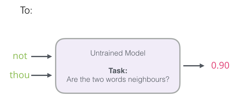
This simple switch transforms the model we need from a neural network to a logistic regression model, making it simpler and faster to compute.
This switch requires us to change the structure of the dataset – the labels are now a new column with values of 0 or 1. Since all the words we added are neighbors, they will all be 1.

Now we can compute at an amazing speed, processing millions of examples in minutes. However, we still need to address a loophole. If all our examples are positive cases (target is 1), we run the risk of facing a clever model that always returns 1 – achieving 100% accuracy without learning anything and generating garbage embedding vectors.
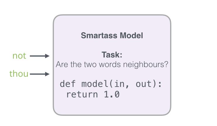
To solve this problem, we need to introduce negative samples into our dataset – word samples that are not neighbors. Our model needs to return 0 for these samples. Now, this is a challenge where the model must work hard to solve the problem, but it can still compute at high speed.
For each sample in our dataset, we add negative examples. They have the same input word, with labels of 0.
But what do we fill in as output words? We randomly draw words from the vocabulary.
The inspiration for this idea comes from noise-contrastive estimation. We compare the actual signal (positive examples of neighboring words) with noise (randomly selected words that are not neighbors). This leads to a huge trade-off in computational and statistical efficiency.
Noise Contrastive Estimation
http://proceedings.mlr.press/v9/gutmann10a/gutmann10a.pdf
Skipgram with Negative Sampling (SGNS)
We have now introduced two (pairs of) core ideas in Word2Vec: negative sampling and skipgram.

Word2Vec Training Process
Now that we understand the two core ideas of skipgram and negative sampling, we can delve deeper into the actual training process of Word2Vec.
Before the training process begins, we preprocess the text to be trained. In this step, we determine the size of the vocabulary (which we call vocab_size and can think of as, for example, 10,000) and the words that belong to that vocabulary.
At the start of the training phase, we create two matrices – the embedding matrix and the context matrix. Both matrices have embeddings for each word in the vocabulary (thus vocab_size is one of their dimensions). The second dimension is how long we want each embedding to be (embedding_size – 300 is a common value, but we saw embeddings of length 50 in earlier examples).
At the start of the training process, we initialize these matrices with random values. Then we begin the training process. In each training step, we choose a positive example and its related negative examples. Let’s look at our first set of examples:
Now we have four words: the input word is “not,” and the output/context word is “thou” (the actual neighbor), along with “aaron” and “taco” (the negative examples). We continue to look up their embedding vectors – for the input word, we look in the embedding matrix; for the context word, we look in the context matrix (although both matrices provide embedding vectors for each word in the vocabulary).
Then, we perform a dot product operation between the input embedding vector and each context embedding vector. In each case, this produces a number that indicates the similarity between the input embedding vector and the context embedding vector.

Now we need a way to convert these scores into probabilities that resemble probabilities – we need to convert them to positive values and ensure they fall within the range of 0 to 1. This is exactly the task that the sigmoid function (logistic function) is well-suited for.
Now we can treat the output of the sigmoid operation as the model’s output for these examples. We can see that before and after the sigmoid operation, “taco” has the highest score, while “aaron” has the lowest.
Since the untrained model has made predictions and we have an actual target label for comparison, let’s calculate how far off the model’s predictions are from the actual labels. To do this, we simply subtract the sigmoid scores from the target labels.
error = target – sigmoid_scores
This is the “learning” part of “machine learning.” We can now use this error score to adjust the embedding vectors of