

Machine Learning Algorithms and Natural Language Processing Recommendations
Source: https://zhuanlan.zhihu.com/p/58425003
Author: Xiao Chuan Ryan
[Introduction to Machine Learning Algorithms and Natural Language Processing]BERT did not come out of nowhere; this article introduces some thoughts on how to derive it from Word2Vec!
Recently, my work has been closely related to pre-trained models, but I found that I had forgotten some details about several word vectors. Therefore, I plan to write an article to refresh my memory and also make it convenient for myself and others to refer to in the future.
1. Language Models
n-gram model
When discussing word vectors, we must start with language models. The traditional statistical language model calculates the probability distribution P(w1, w2, …, wm) for a sentence of length m, representing the likelihood of that sentence existing. This probability can be calculated using the following formula:
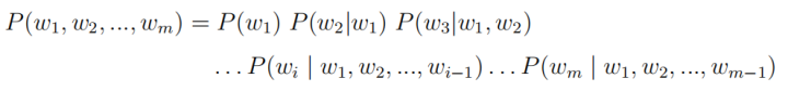
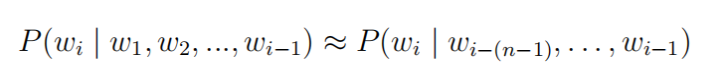
However, in practice, estimating becomes very difficult as the length of the sentence increases. Therefore, the n-gram model simplifies the above calculation: it assumes that the occurrence of the i-th word only depends on the previous n-1 words, i.e.:
In actual calculations, the probability is usually estimated based on the frequency of n-grams appearing in the corpus:
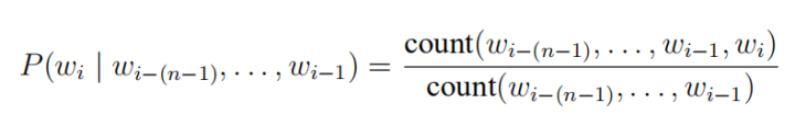
To retain the original order information of the sentence, we certainly want n to be as large as possible, but in reality, when n is slightly larger, the frequency of that n-gram appearing in the corpus will decrease, leading to data sparsity issues in the estimated probabilities. The emergence of neural network language models effectively solves this problem.
Neural Network Language Model
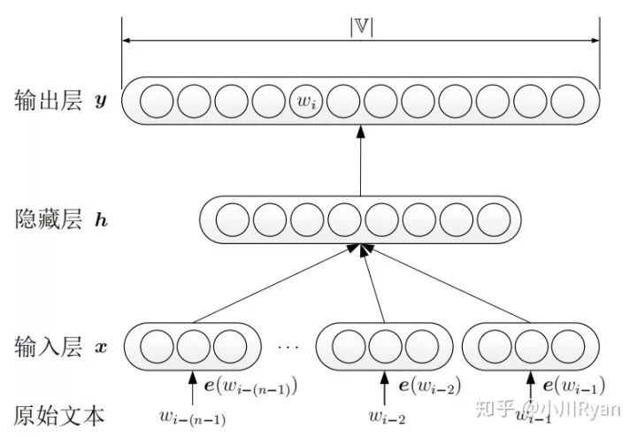
The neural network language model does not use frequency to estimate the probability of n-grams but instead trains a language model through a neural network.
First, the original text is one-hot encoded, then multiplied by the word embedding matrix to obtain the vector representation of each word, which is concatenated as the input layer. The output layer adds a softmax to convert y into the corresponding probability value. The model uses stochastic gradient descent to maximize
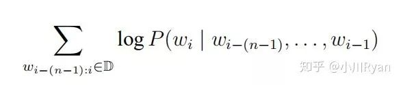
the result.
Recurrent Neural Network Language Model (RNNLM)
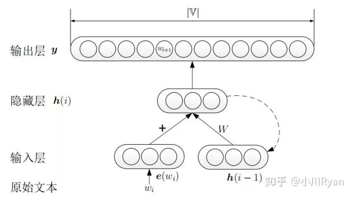
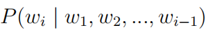
Although NNLM uses a neural network to predict the likelihood of sentences, it still simplifies the computation using n-grams, whereas RNNLM directly models the entire sentence, i.e., directly calculates
The difference between RNNLM and NNLM lies in the computation of the hidden layers:
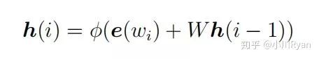
Each node in the hidden layer relies on both the input of the current word’s vector and the output of the previous word’s hidden state, allowing the model to learn and predict using more complete contextual information.
The purpose of the above-mentioned NNLM and RNNLM is to establish a language model, and the word vectors (i.e., the word embedding matrix before the input layer) are merely a byproduct of the entire process. Starting from C&W, models were constructed with the direct goal of generating word vectors. Since CBOW is an upgrade and simplification based on C&W, we will start with CBOW.
2. Word2Vec
CBOW
The main idea of CBOW is to predict a word in a sentence by using its context. Let’s first look at a simple case where there is only one word in the context (i.e., using one word to predict a center word):
The input layer is the one-hot encoding of the context word, with the vocabulary size V, and the first weight matrix W is a word vector matrix with V rows and N columns, where N is the dimension of the word vectors, such as commonly used 300-dimensional, 400-dimensional, etc. We temporarily call W the “input word vector,” which serves to represent the context word’s vector, such as
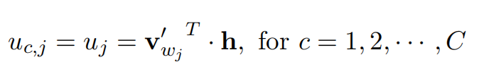
Here, the hidden layer does not go through a nonlinear activation but simply passes the dimensions of the context word’s vector represented by W linearly to the next layer; the matrix W’ is the transposed result of W, temporarily called the “output word vector,” which serves to represent the vector of the center word to be predicted; what we need to do now is calculate the “score” for all words in the vocabulary and select the center word with the highest probability as the prediction result.
The method used in the paper is to take the dot product of the context word’s vector and the center word’s vector to represent the score, i.e.
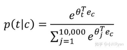
We know that the result of the dot product of two vectors can reflect their similarity, which I believe is why word vectors are very effective for similar word detection. By multiplying the hidden layer with , we can obtain the scores of all words in the vocabulary with the context words, and finally, the softmax function is calculated in the output layer to normalize the scores into probabilities:
The center word with the highest probability is taken as the predicted result. The training process uses backpropagation and stochastic gradient descent to continuously update the word vector matrix, and finally, “input word vector” is usually selected as the final result.
Next, let’s look at CBOW with multiple words in the context.
Using C context words to predict the center word differs from the case with only one word in that the hidden layer no longer takes the dimensions of one word’s vector but rather the average of the dimensions of the C context words’ vectors, i.e.
Other aspects are not significantly different; minimizing the loss function results in the optimal word vectors.
For detailed training step derivation, please refer to the paper “word2vec Parameter Learning Explained”. The derivation in the paper is very detailed and even includes a review of backpropagation for beginners in the appendix. After all, what we learn in a cursory manner is ultimately just a house of cards, so I strongly recommend reading and experiencing the derivation process in the paper carefully.
Skip-gram
Conversely, the main idea of Skip-gram is to select a certain word (also known as the center word) in a sentence and use it to predict other words in the context.
The input layer is the one-hot encoding of the center word, which is transformed into its vector representation through the “input word vector”; the hidden layer consists of the dimensions of the center word’s vector:
The difference in Skip-gram is that the output layer needs to calculate C distributions (C is the number of context words to be predicted) by calculating the maximum probability word in each distribution to determine the most likely C words. The C distributions share the same “output word vector” and similarly calculate the scores of all words in each distribution:
Then minimize the loss function
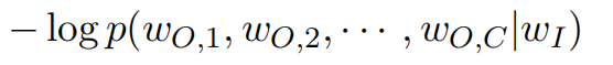
to obtain the optimal word vectors.
3. Optimization Methods
In the unoptimized CBOW and Skip-gram, the output layer uses a general softmax layer, and when predicting the probability of each word, it requires summing the normalization term of the denominator each time, while the complexity of exponentiation is relatively high. Therefore, when the vocabulary size is large, the prediction efficiency will be extremely low. Both CBOW and Skip-gram have corresponding optimization methods to reduce computational complexity; we will introduce two of them.
Hierarchical Softmax
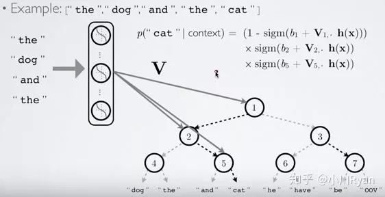
First, we construct a Huffman tree using the occurrence count (or frequency) of each word in the vocabulary as weights, where the leaf nodes represent the one-hot representation of each word in the vocabulary, and each non-leaf node is also represented as a vector. At this point, the path from the root node to each leaf node can be represented by a series of Huffman codes. For example, assuming the left node is 0 and the right node is 1, “cat” in the above figure can be represented as 01.
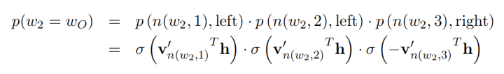
During the prediction process, each non-leaf node uses its own vector representation to perform binary classification (e.g., using logistic regression), and the classification result directs whether to go to the left or right node. In this way, the probability of predicting “cat” can be represented as P(node1==0)*P(node5==1), and more complex tree structures follow similarly. This method significantly improves prediction efficiency when predicting the probability of a specific word.
Now, let’s look at the formal explanation in the paper:
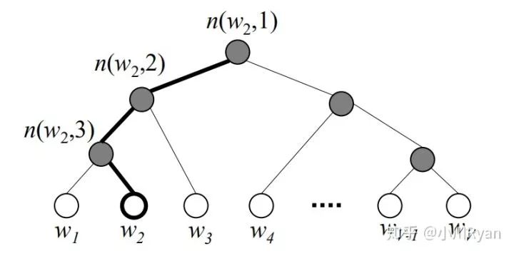
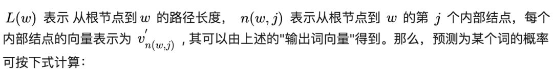
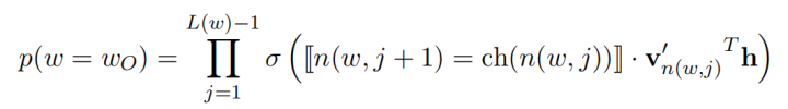
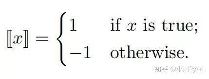
The function [[x]] is defined as:
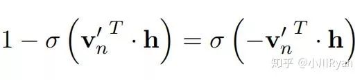
ch(n) denotes the left child of node n, and h is the output of the hidden layer. The probability of going left at an internal node is defined as
and the probability of going right is
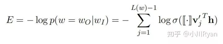
Minimizing the loss function
For detailed formula derivation, please refer to the blog:
https://blog.csdn.net/itplus/article/details/37969979
Negative Sampling
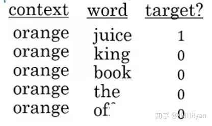
The purpose of negative sampling is still to improve the high computational cost problem caused by the need to sum the normalization term for predicting the probability of each word using ordinary softmax. Its core idea is to transform the prediction of the probability of each word into a small-scale supervised learning problem. Specifically, for a sentence in the corpus, such as “I want a glass of orange juice to go along with my cereal,” we select “orange” as the context and mark “juice” as 1 (i.e., a positive sample), then select k other words from the sentence as negative samples. For example, if k=4, it looks like this:
We then use these sampled examples to train a logistic regression model. In this way, when predicting the probability of the word “orange” appearing in the context, although it still requires multiple iterations to see which word has the highest probability, during each iteration, the calculation of softmax:
The normalization term in the denominator no longer needs to sum all words in the vocabulary as in the previous formula but only needs to sum the 5 sampled words, greatly improving training efficiency. As for the selection of k, Mikolov’s paper mentions that for smaller-scale corpora, k is generally chosen between 5 to 20, while for larger scales, it is kept under 5.
The key is how to sample?
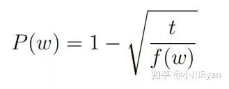
If sampling according to the observed distribution of word frequencies, it is likely to sample words like “a”, “the”, “of”, etc., which do not carry much practical significance. Therefore, the paper proposes the idea of subsampling: if the frequency of word w exceeds a certain threshold t, then with a probability of P(w), this word is skipped during sampling:
In actual training, there is also a small trick: let f(wi) be the observed probability of word wi in the vocabulary, then sample wi with a probability of P(wi):
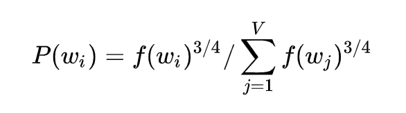
As for why this value works better, there is no corresponding theoretical proof.
For detailed derivation of the negative sampling training process, please refer to the blog:
https://blog.csdn.net/itplus/article/details/37998797
This topic will be published in three parts; the next will detail GloVe and FastText, and the following will introduce ELMo, GPT, and BERT.
Stay tuned
References
[1] Xin Rong, word2vec Parameter Learning Explained
[2] Lai Siwei, Research on Word and Document Semantic Vector Representation Methods Based on Neural Networks
[3] Tomas Mikolov, Distributed Representations of Words and Their Compositionality
[4] Blog: Mathematical Principles in Word2Vec
Click the original link to visit the author’s Zhihu column!
Fan Benefits

To facilitate interaction with fans
We have established a Python algorithm learning and machine learning algorithm group
👉 We are committed to Python algorithm learning and machine learning algorithms. The group shares knowledge daily, including but not limited to machine learning resources, company referrals, Leetcode problem-solving guides, etc.
👉 There are many CV and NLP experts in the group, some working in large companies, while others are pursuing master's/Ph.D. degrees. If you have any questions, you can communicate in the group, and we can progress together!
👉 No promotional messages are allowed in the group; the focus is on discussion and exchange. The public account owner does not need to join; thank you!

If the group is full, please scan the code to contact the administrator
Note: "School/Organization - Name"

Recommended Reading:
Here are some Python and algorithm technology experts

A discussion: How to explain to my girlfriend why the delivery address cannot be modified on Double 11

All major AI international academic conferences in 2019 are here; please check it out!