Illustrated Guide to Transformers

Step 1 — Define the Dataset

For demonstration purposes, the dataset here contains only three English sentences, using a very small dataset to intuitively perform numerical calculations. In real applications, larger datasets are used to train neural network models, such as ChatGPT, which was trained on data amounting to 570 GB.

Our entire dataset contains only three sentences.

Since the dataset is small, the data cleaning workload is also relatively small. However, cleaning 570 GB of data would be a very tedious task.

Step 2 — Determine Vocabulary Size

The vocabulary size determines the total number of unique words in the dataset. The following formula can be used to calculate it, where N is the total number of words in the dataset.

vocab_size formula, where N is the total word count.

The dataset needs to be broken down into individual words, and then the word count N needs to be calculated.

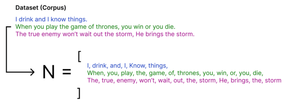
After obtaining N, remove duplicates and then count the number of unique words to determine the vocabulary size.

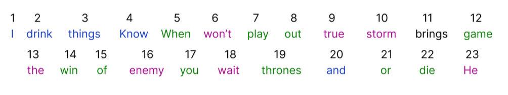
Thus, the vocabulary size is 23, because there are 23 unique words in our dataset.

Step 3 — Encoding

Now, we need to assign a unique number to each unique word.

Since we treat individual tokens as single words and assign a number to them, currently some large models use the following formula to treat part of a word as a single token: 1 Token = 0.75 Word

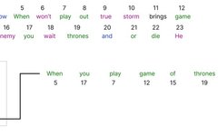
After encoding the entire dataset, it’s time to select our input and start using the transformer architecture.

Step 4 — Calculate Embeddings

We select a sentence from the corpus and process it with the transformer architecture.

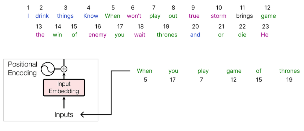
We have selected the input, and next we need to calculate an embedding vector for it. The original paper used a 512-dimensional embedding vector for each input word.

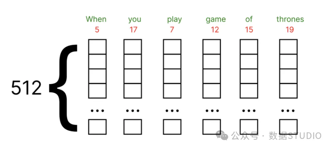
Here, for convenience of demonstration, we use a smaller dimensional embedding vector to visualize the calculation process. We choose a dimension of 6 for the embedding vector.

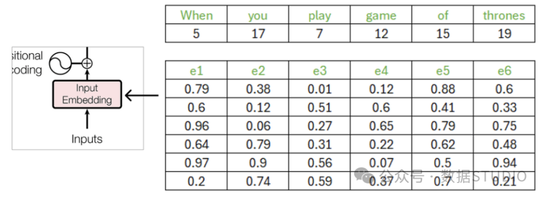
The values of the embedding vector are between 0 and 1 and are initialized randomly at the start (random initialization). As the transformer begins to understand the meanings between words, the embedding vectors will also be updated accordingly.

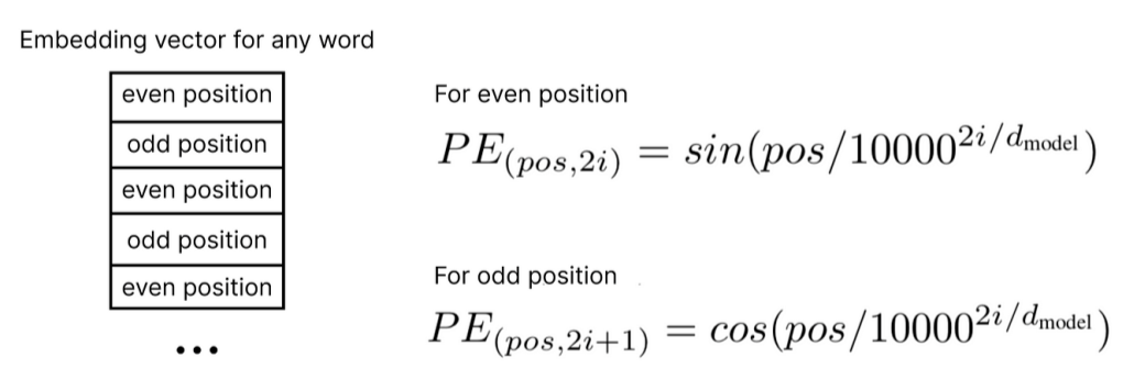
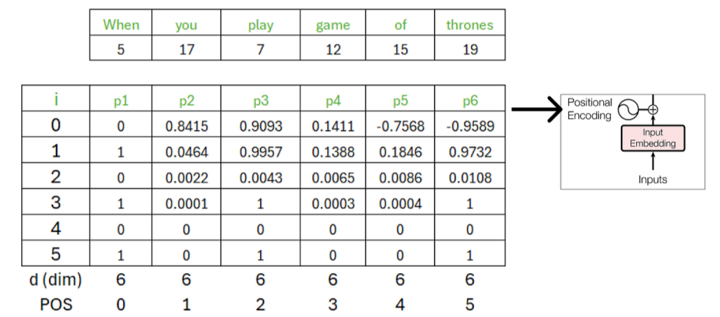
Step 5 — Calculate Positional Embeddings

Now we need to calculate the positional embeddings for the input. There are two formulas for positional embeddings, depending on the position of the i-th value of each word’s embedding vector.

Our input sentence is “when you play the game of thrones”, the starting word is “when”, the starting index (POS) value is 0, and the dimension (d) is 6, so i ranges from 0 to 5. Thus, we calculate the positional embedding for the first word of the input sentence.

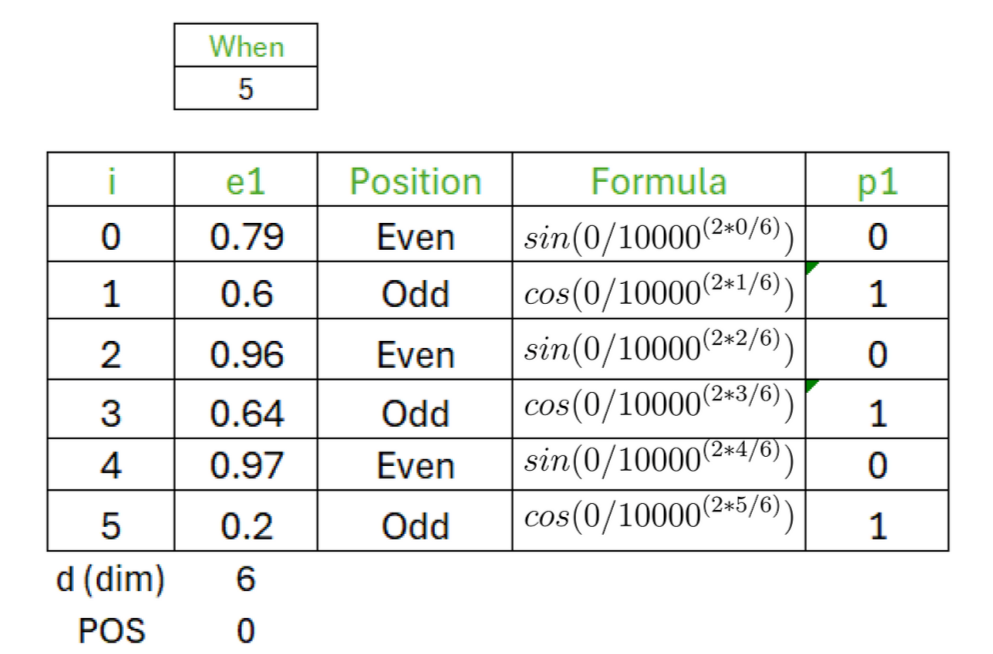
Similarly, we can calculate the positional embeddings for all words in the input sentence.

Step 6 — Combine Position and Word Embeddings

After calculating the positional embeddings, we need to add the word embeddings and positional embeddings together.

The matrix obtained by combining the two matrices (word embedding matrix and positional embedding matrix) will be treated as the input to the encoder part.

Step 7 — Multi-Head Attention

Multi-head attention consists of many single-head attentions, with each single-head attention responsible for different information extraction and focus points. The multi-head attention technique maps the input sequence to a set of virtual query, key, and value vectors. The vectors obtained from these mappings will be used to calculate attention weights and generate contextual representations. Each head learns different mappings, allowing it to focus on different features.

The number of single-head attentions we need to combine depends on ourselves. For example, Meta’s LLaMA LLM uses 32 single-head attentions in its encoder architecture. Below is a diagram of single-head attention.

Input signal  --->|  Q  |-----\
Input signal  --->|  K  |----MultiHead Attention---> Output |
Input signal  --->|  V  |-----/

There are three inputs: query, key, and value.

Each matrix is obtained by multiplying the transposed version of the same matrix calculated previously (by adding the word embedding and positional embedding matrices) with a different set of weight matrices.

The calculation can be done in the following steps:

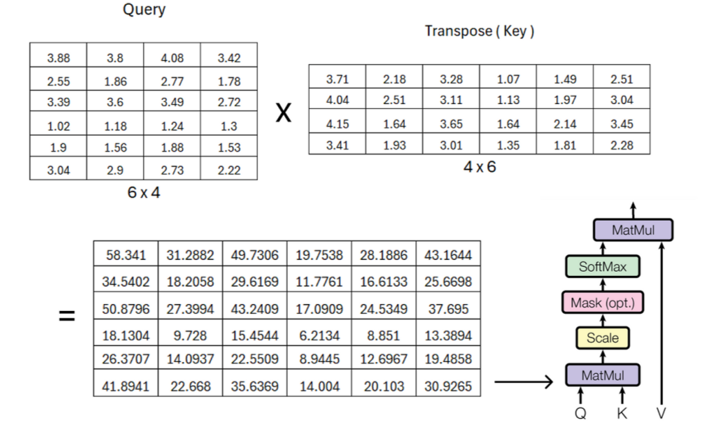
1. Obtain the transposed query matrix and key matrix.
2. Multiply the query matrix by the transposed key matrix to obtain the attention score matrix.
3. Multiply the attention score matrix by the value matrix to obtain the final output matrix.

In actual implementation, you need to use matrix multiplication algorithms to perform these steps. You also need to consider the initialization and learning process of the weight matrices, as well as how to handle the updates of random values in practical applications.

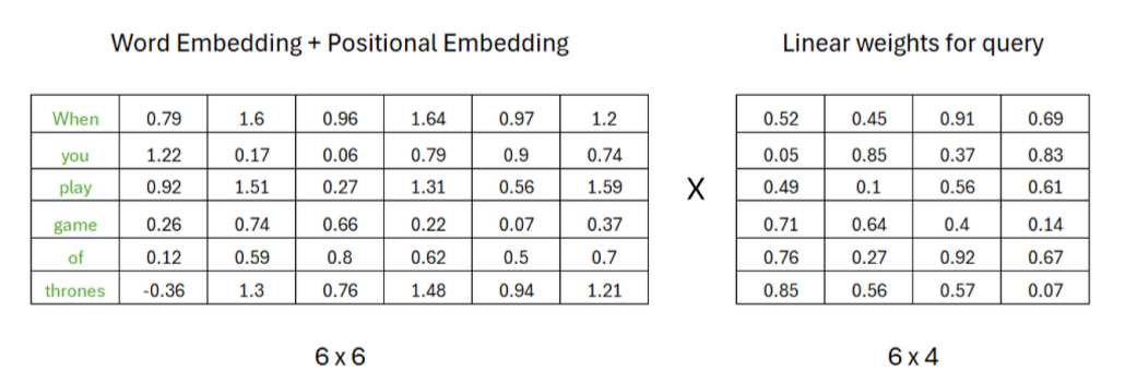
Assuming that to compute the query matrix, the number of rows in the weight matrix must match the number of columns in the transposed matrix, while the number of columns in the weight matrix can be arbitrary; for example, we assume there are 4 columns in the weight matrix. The values in the weight matrix are random 0 and 1, and as our transformer begins to learn the meanings of these words, these values will be updated later.

Similarly, we can calculate the key and value matrices using the same procedure, but the values in the weight matrices must be different.

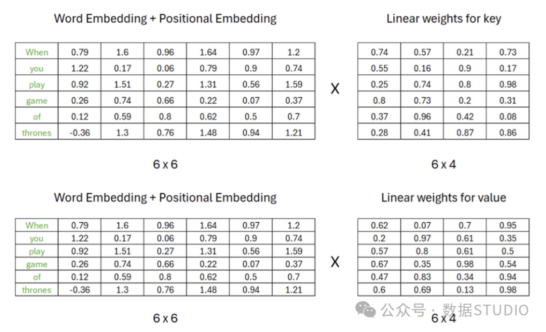
Therefore, after matrix multiplication, we obtain the results for **query , key , and value .**

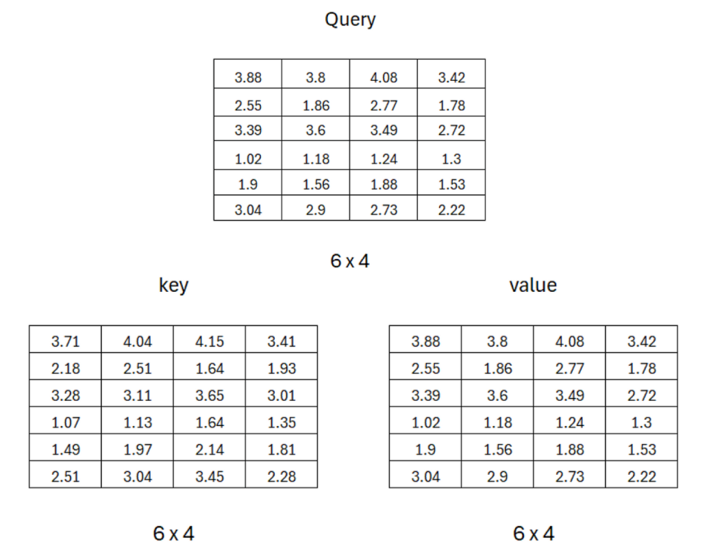
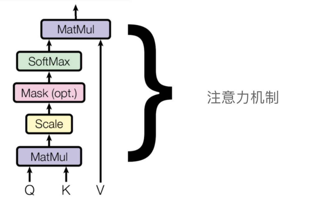
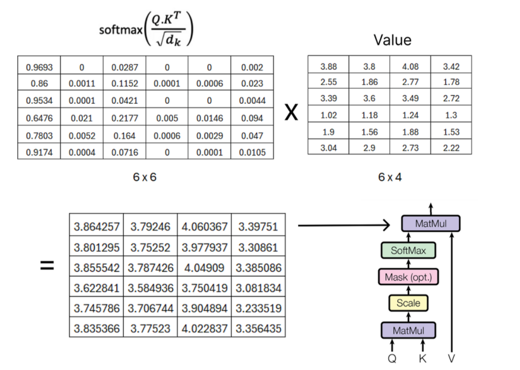
Now that we have all three matrices, we can start calculating single-head attention step by step.

The calculation formula:

To scale the result matrix, we must reuse the dimension of the embedding vector, which is 6.

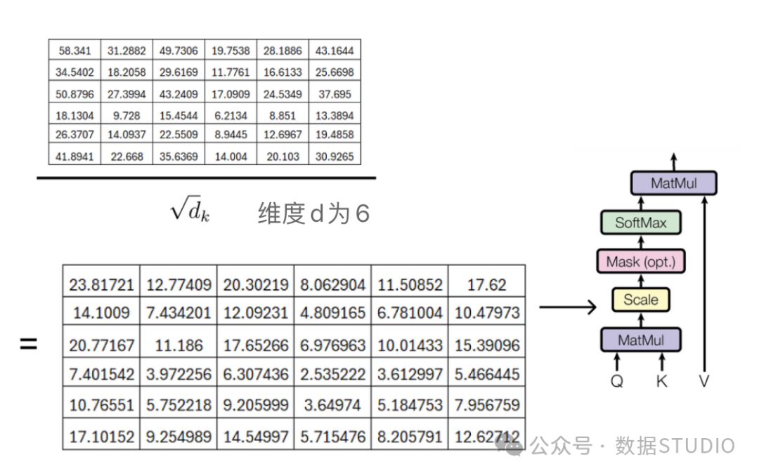
The question arises: why divide by:

This question was roughly answered in the original paper “Attention is All You Need”.

While for small values of the two mechanisms perform similarly, additive attention outperforms dot product attention without scaling for larger values of . We suspect that for large values of , the dot products grow large in magnitude, pushing the softmax function into regions where it has extremely small gradients. To counteract this effect, we scale the dot products by .

The authors say that as the value of increases, the softmax function causes the gradient vanishing problem, so a softmax temperature is set to mitigate this issue. Here, the temperature is set to, which is multiplied by.

This answer is certainly correct, but it will lead to two more questions:

1. Why does it cause gradient vanishing?
2. Why is it , is there a better value?

The first question.

1. If increases, the variance increases.
2. Increased variance causes the differences between elements of the vectors to increase.
3. Increased differences between elements cause softmax to degenerate into argmax, meaning that the softmax value of the maximum becomes 1, while other values become 0.
4. If softmax has only one element equal to 1 and all others equal to 0, the gradient during backpropagation will be 0, which is known as the gradient vanishing.

The second question.

The scale value is actually normalizing to a vector with mean 0 and variance 1.

As for whether it is the best, it is hard to say, because we are not very clear about the distribution of parameters. Su has attempted to solve the best scale values for some common distributions, which can be found here: https://spaces.ac.cn/archives/9812

The next step is Mask, which is optional, we will not calculate it. Using a mask is like telling the model to only pay attention to what happens before a specific time point, rather than peeking into the future when determining the importance of different words in the sentence. This will help the model gradually understand things without cheating by knowing the future.

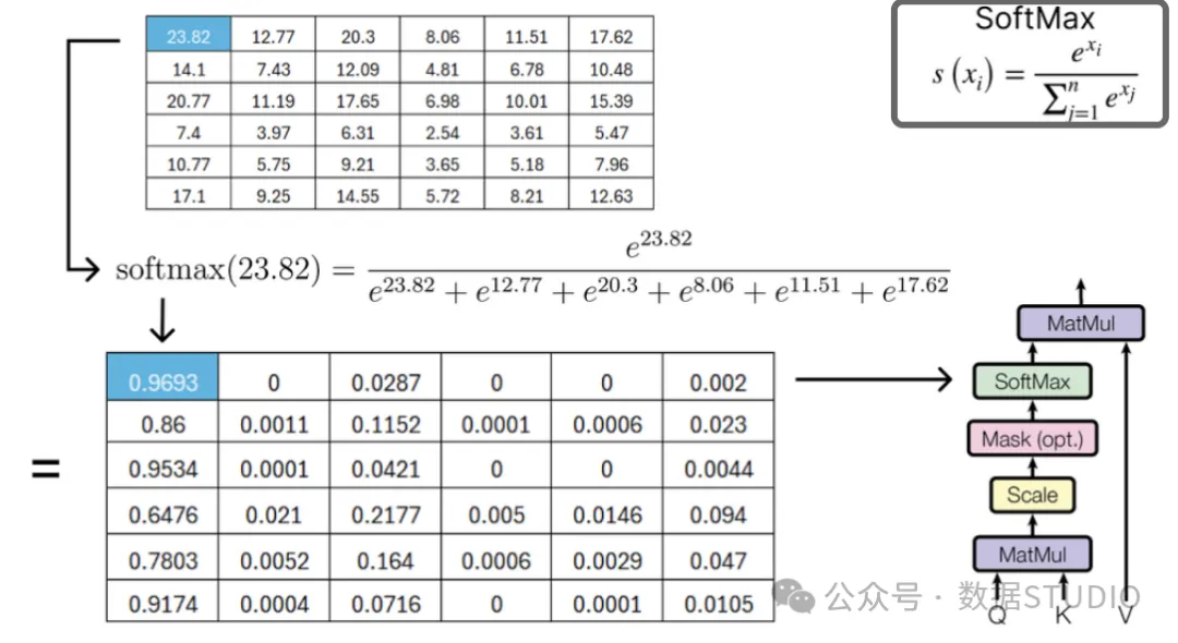
Thus, we will now apply the softmax operation on the scaled result matrix.

The softmax operation is typically used for multi-class problems, mapping the input vector to a probability distribution such that each element of the vector is between 0 and 1, and all elements sum to 1. This helps the model output probabilities for each category.

Perform the final multiplication step to obtain the result matrix of single-head attention.

Multi-head attention consists of multiple single-head attentions, visualized as follows:

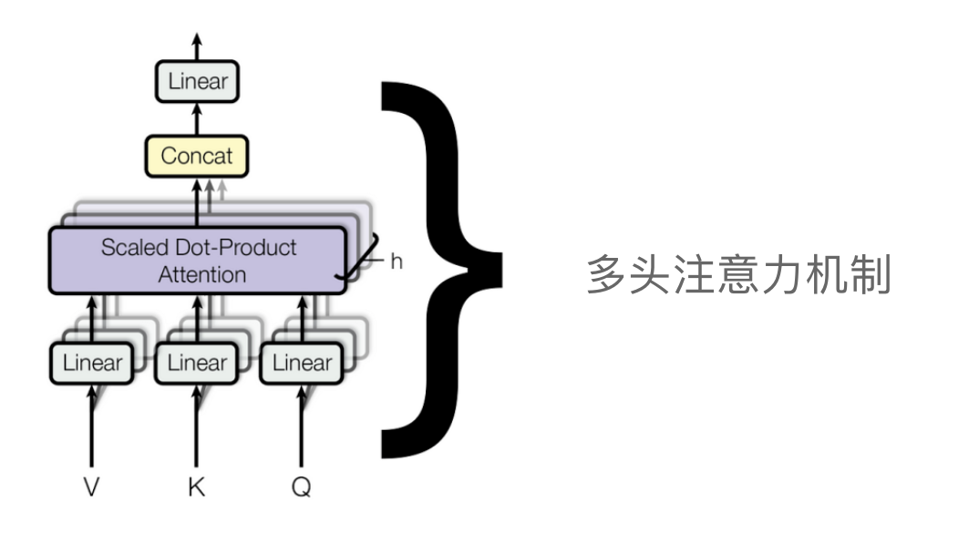Multi-head attention mechanism in Transformer

Each single-head attention mechanism has three inputs: query, key, and value, each with a different set of weights. Once all single-head attention mechanisms output their result matrices, they will all be concatenated, and the final concatenated matrix will again undergo a linear transformation by multiplying it with a set of randomly initialized weight matrices, which will later be updated during the training of the Transformer.

The result matrix obtained from multi-head attention is derived from the computation of multiple attention weights on the original input matrix, where each attention weight corresponds to a different “head”. The purpose of adding these result matrices to the original matrix is to integrate the information from multiple attention heads, thereby better capturing the complex relationships and features within the input data. This summation operation enhances the model’s ability to model the correlations and complexities between different inputs, improving the model’s performance and robustness.

In our example, the use of multi-head attention is illustrated as shown below.

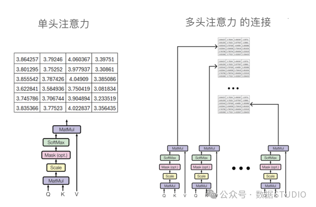Single-head attention mechanism vs multi-head attention mechanism

Whether it is single-head attention or multi-head attention, the result matrix needs to undergo another linear transformation by multiplying it with a set of weight matrices.

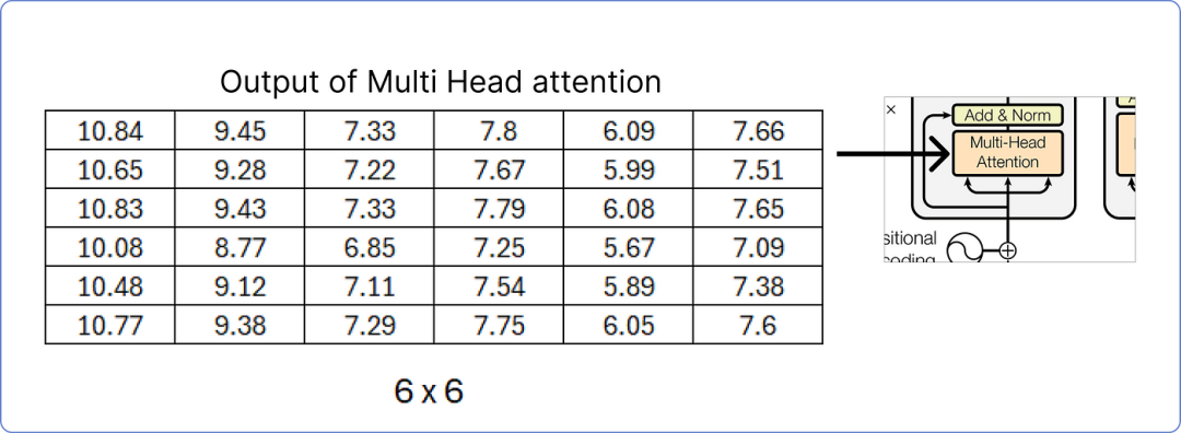
Ensure that the number of columns in the linear weight matrix must equal the number of columns in the matrix calculated earlier (the word embedding + positional embedding matrix), because in the next step, we will add the normalized result matrix to the (word embedding + positional embedding) matrix.

Step 8 — Residual Connection and Normalization

The result matrix obtained from multi-head attention is added to the original matrix.

The purpose of adding the result matrix obtained from multi-head attention to the original matrix is to enhance the model’s ability to learn and understand critical information. In the multi-head attention mechanism, computing multiple sets of different attention weights allows the model to better capture the correlated information and context within the input data, improving the model’s expressive capability.

By adding the result matrix obtained from attention calculations to the original matrix, we can combine the information in the original matrix with the important information obtained from attention, enabling the model to better utilize significant information for learning and prediction, thereby enhancing the model’s performance and generalization ability. This operation increases the model’s perception of the relevance and importance within the input data, improving its processing effectiveness.

Next, we perform normalization on the added matrix, calculating the mean and standard deviation for each row.

Layer Normalization is used to normalize the output of each attention mechanism layer to help the model converge faster and reduce the issues of gradient vanishing or explosion.

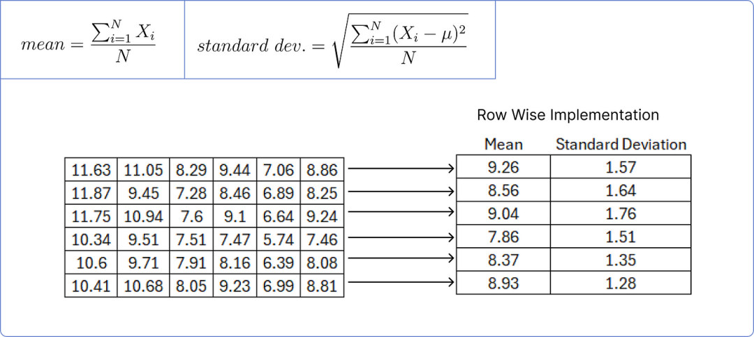
We subtract the corresponding row mean from each value in the matrix and then divide by the corresponding standard deviation.

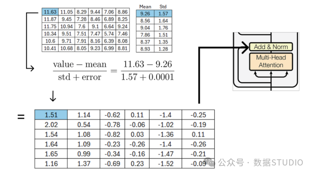
In the self-attention mechanism of the transformer model, to avoid division by zero and prevent the entire term from becoming infinite, a small error value (e.g., 1e-6) is usually added to the denominator during normalization. This small error value ensures numerical stability and prevents numerical computation errors due to zero denominators.

Step 9 — Feed Forward Network

After normalizing the matrix, it will be processed through a feed-forward network. We will use a very basic network that consists of only one linear layer and one ReLU activation function layer.

First, we need to calculate the linear layer by multiplying the last computed matrix with a set of randomly initialized weight matrices that will be updated during the training of the transformer, and then add the result matrix to a bias matrix also containing random values.

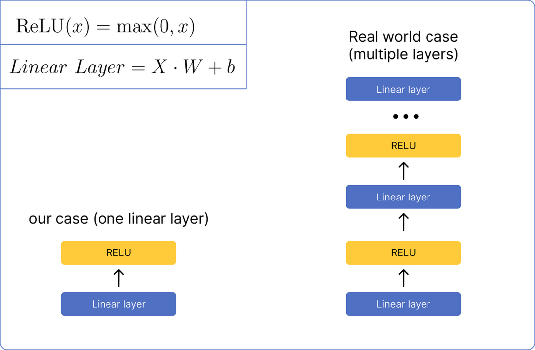
After calculating the linear layer, we need to pass it through the ReLU layer and use its formula.

Step 10 — Residual Connection and Normalization Again

Once we obtain the result matrix from the feed-forward network, we need to add it to the matrix obtained from the previous residual connection and normalization step, and then normalize it using row mean and standard deviation.

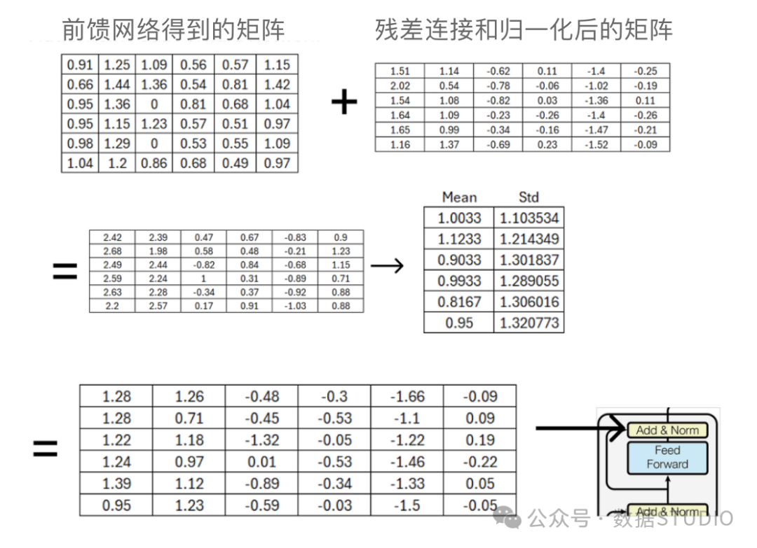Feed forward network after Add & Norm

The output matrix from this residual connection and normalization step will serve as the Query and Key matrices in one of the multi-head attention mechanisms present in the decoder part, which can be easily understood by tracing back from the residual connection and normalization to the decoder part.

Step 11 — Decoder Part

So far, we have calculated all the steps of the encoder part, from encoding the dataset to passing the matrix to the feed-forward network.

The encoder is responsible for converting the input sequence into hidden representations. Each transformer encoder essentially consists of a stacked structure made up of multiple encoder layers, each encoder layer consisting of two sub-layers: multi-head self-attention mechanism and fully connected feed-forward neural network.

1. Multi-head self-attention mechanism: used to capture the correlations between different positions in the input sequence. This layer can simultaneously compute the attention weights between each element in the input sequence to encode the information of each position. It allows the model to consider all positions in the input sequence simultaneously and learn the dependencies between different positions. In the self-attention mechanism, each element of the input sequence will compute attention with all other elements, resulting in a representation for each element.
2. Fully connected feed-forward neural network: used to learn richer feature representations for each position. This layer independently transforms the hidden representation for each position, followed by residual connection and layer normalization. This sub-layer applies two linear transformations and an activation function to the representation of each position in the encoder layer, converting the input into more abstract representations.

The function of the encoder is to transform the input sequence into a series of hidden representations that contain the semantic and contextual information of the input sequence. These hidden representations can be used by the subsequent decoder to generate the target sequence or perform other tasks, such as language modeling, machine translation, etc.

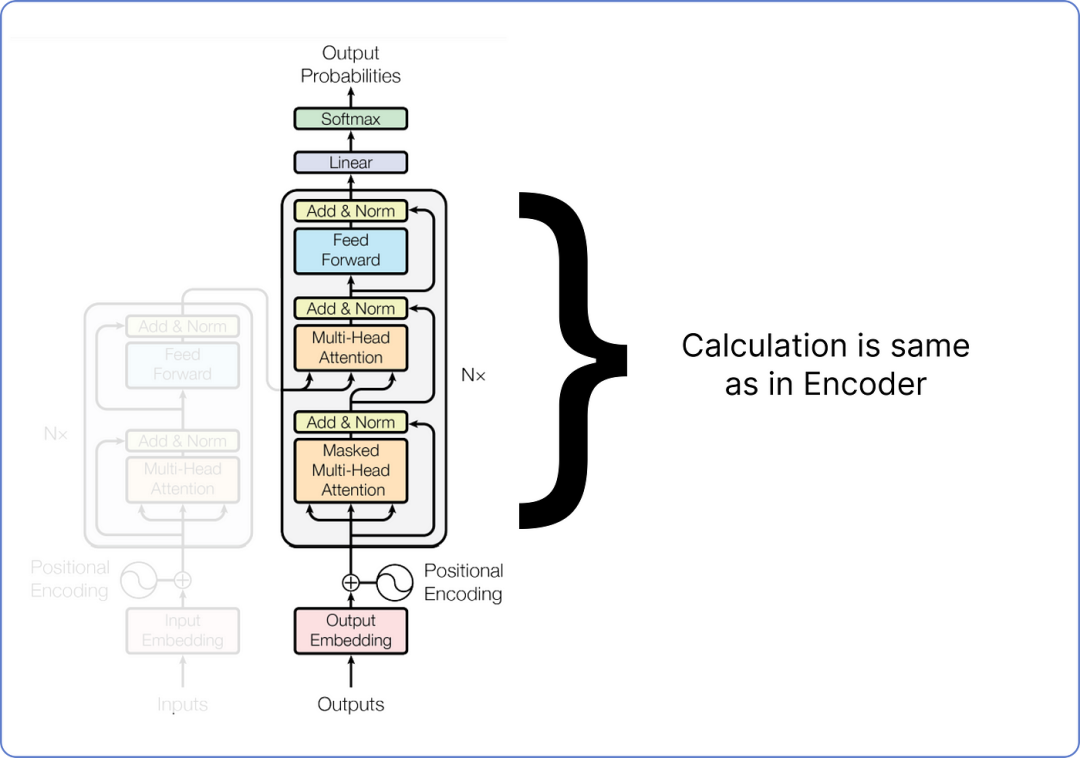
The decoder part of the transformer will involve similar matrix multiplications.

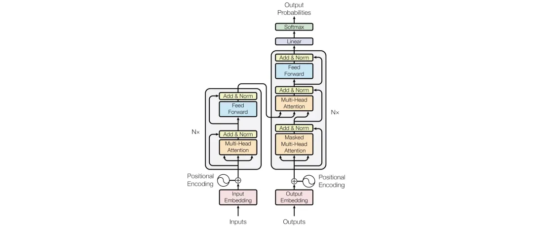
Let’s take a look at our transformer architecture. So far, we have covered what we have and what we still need to cover:

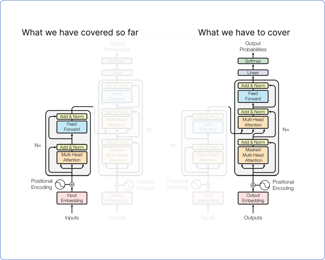
We will not compute the entire decoder, as most of its parts involve calculations similar to what we have already done in the encoder. Detailing the calculations of the decoder would only make this document lengthy due to repetitive steps. Instead, we only need to focus on the computations of the inputs and outputs of the decoder.

During training, the decoder has two inputs. One comes from the encoder, where the output matrix from the last residual connection and normalization serves as the Query and Key for the second multi-head attention layer in the decoder part. Below is its visualization (from batool haider):

And the Value matrix comes from the result of the decoder after the first residual connection and normalization step.

The second input for the decoder is the predicted text. If you remember, our input to the encoder was when you play game of thrones, so the input to the decoder is the predicted text, which in our case is you win or you die.

However, the predicted input text needs to follow standard tokens to let the transformer know where to start and where to end.

Where <start> and <end> are two new tokens introduced. Additionally, the decoder only accepts one token as input at a time. This means that <start> will be the input, and you must be its predicted text.

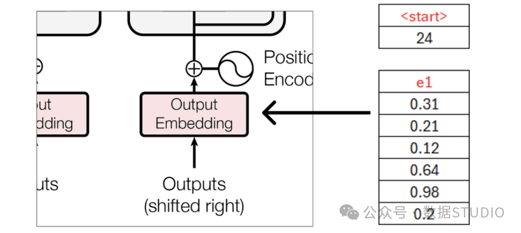
We already know that these embeddings are filled with random values, which will be updated during training.

We calculate the remaining blocks in the same way as we did in the encoder part.

Before delving into more details, we need a simple mathematical example to understand what Mask multi-head attention is.

Step 12 — Understanding Mask Multi-Head Attention Mechanism

In the Transformer, Mask multi-head attention acts like a spotlight, helping the model focus on different parts of the sentence. It is special because it prevents the model from cheating by looking at words behind the sentence. This helps the model gradually understand and generate sentences, which is crucial for tasks like conversations or translating words into another language.

Suppose we have the following input matrix, where each row represents a position in the sequence, and each column represents a feature:

Input matrix for masked multi-head attention

Now, let’s understand the Mask multi-head attention component with two heads:

1. Linear Projections (Query, Key, Value): Assume the linear projections for each head are: Head 1: Wq1, Wk1, Wv1 and Head 2: Wq2, Wk2, Wv2
2. Calculate Attention Scores: For each head, use the dot product of the query and key to compute the attention scores, applying the mask to prevent focusing on future positions.
3. Apply Softmax: Apply the softmax function to obtain the attention weights.
4. Weighted Sum (Value): Multiply the attention weights by the values to obtain the weighted sum for each head.
5. Concatenate and Linear Transformation: Concatenate the outputs of the two heads and apply a linear transformation.

Let’s perform a simple calculation:

Assume there are two conditions

• Wq1 = Wk1 = Wv1 = Wq2 = Wk2 = Wv2 = I, that is, the identity matrix.
• Q = K = V = input matrix

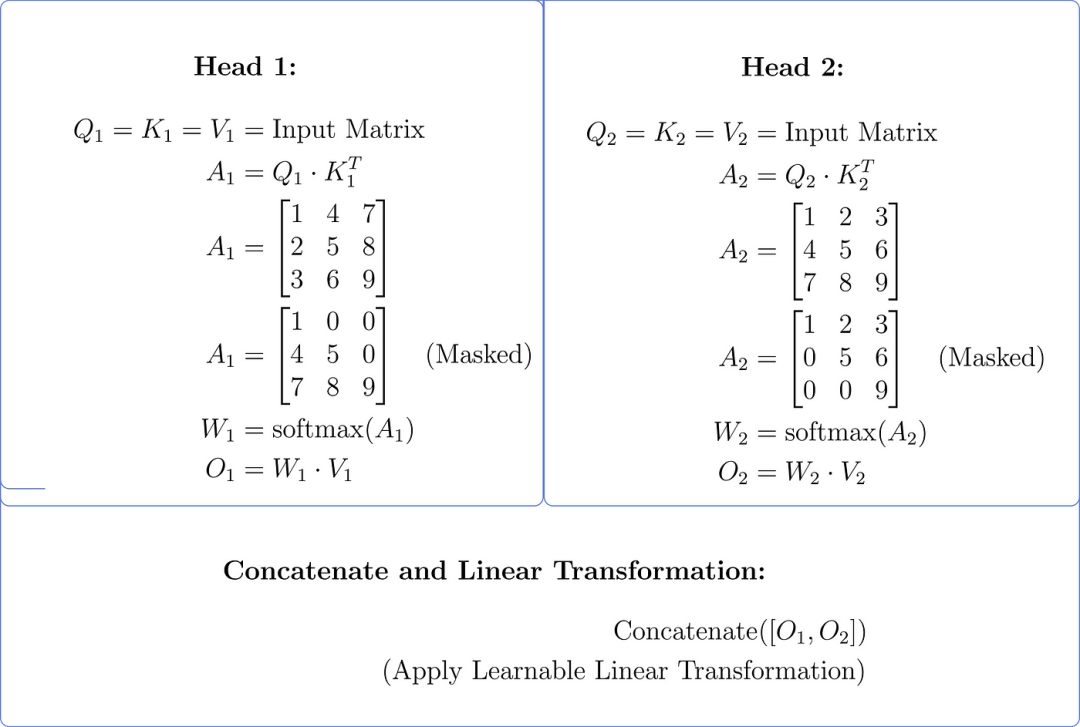
The concatenation step combines the outputs of the two attention heads into a single set of information. Imagine you have two friends who each give you advice on a question. Combining their suggestions means putting both pieces of advice together so that you get a more comprehensive understanding of what they suggest. In the context of the Transformer model, this step helps capture different aspects of the input data from multiple perspectives, providing the model with richer representations for further processing.

Step 13 — Calculate Predicted Words

The output matrix from the last addition and normalization block of the decoder must have the same number of rows as the input matrix, while the number of columns can be arbitrary. Here we use 6.

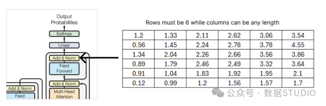
Output from the decoder’s residual connection and normalization

The final residual connection and normalization block output matrix of the decoder must be flattened to match with the linear layer to find the predicted probabilities for each unique word in our dataset (corpus).

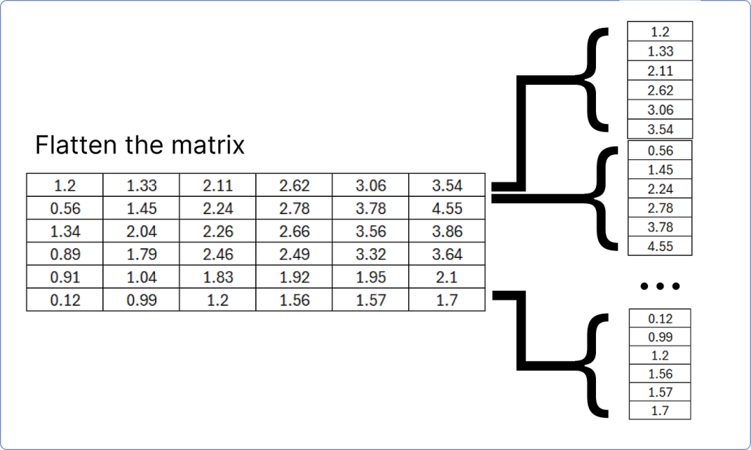
This flattened layer will compute the logit (scores) for each unique word in the dataset through the linear layer.

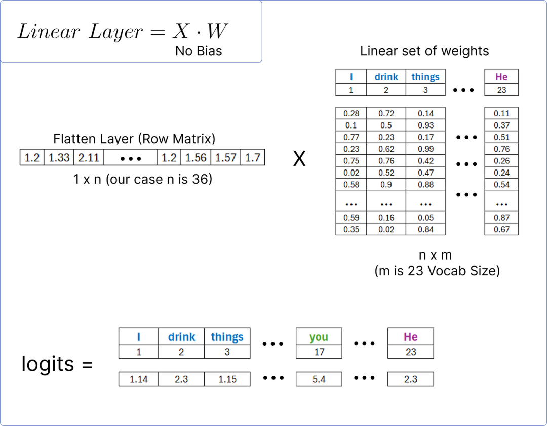
Once we obtain the logits, we can use the softmax function to normalize them and find the word with the highest probability.

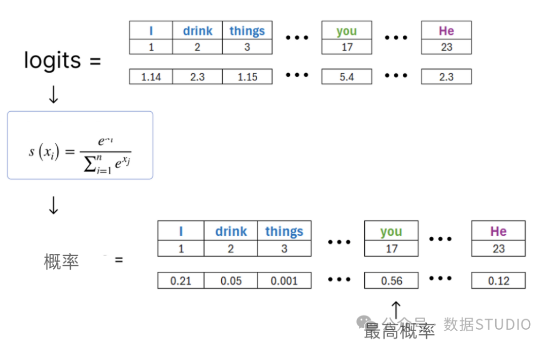Finding the predicted word

Thus, according to our calculations, the predicted word from the decoder is you.

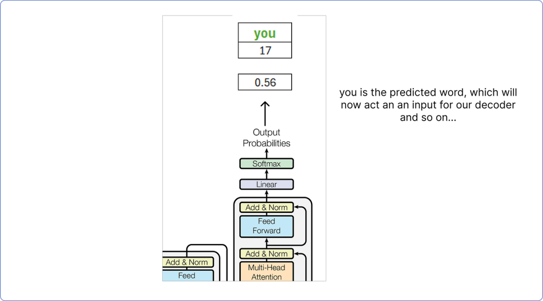
This predicted word you will be treated as the input word for the decoder, and this process continues until the <end> token is predicted.

Key Points

1. The above example is simple and easy to understand, not involving specific periods or requirements for other programming languages, and can be visualized using Python, etc.
2. This example demonstrates the training process and points out that it is difficult to evaluate or test intuitively through matrix methods.
3. Using masked multi-head attention prevents the transformer from observing the future, helping to avoid overfitting the model.

Final Thoughts

In this article, I demonstrated how to perform basic mathematical operations using matrix methods. In addition to introducing positional encoding, softmax, and feed-forward networks, the most critical aspect is multi-head attention.

Source: Data STUDIO