Hands-On Series with Hugging Face Transformers – 03 Analysis of Transformers Model

In Chapter 2, we saw what is needed to fine-tune and evaluate a Transformer. Now let’s take a look at how they work under the hood. In this chapter, we will explore the main components of the Transformer model and how to implement them using PyTorch. We will also provide guidance on how to do the same in TensorFlow. We will first focus on establishing the attention mechanism, then add the necessary components to make the Transformer encoder work. We will also briefly touch on the structural differences between encoder and decoder modules. By the end of this chapter, you will be able to implement a simple Transformer model yourself!

While a deep technical understanding of the Transformer architecture is not usually a prerequisite for using Transformers and fine-tuning models for your use case, it is helpful for understanding and navigating the limitations of Transformers and using them in new domains.

This chapter also introduces the taxonomy of Transformers to help you understand the various models that have emerged in recent years. Before diving into the code, let’s first outline the original architecture that sparked the Transformer revolution.

Transformers Architecture

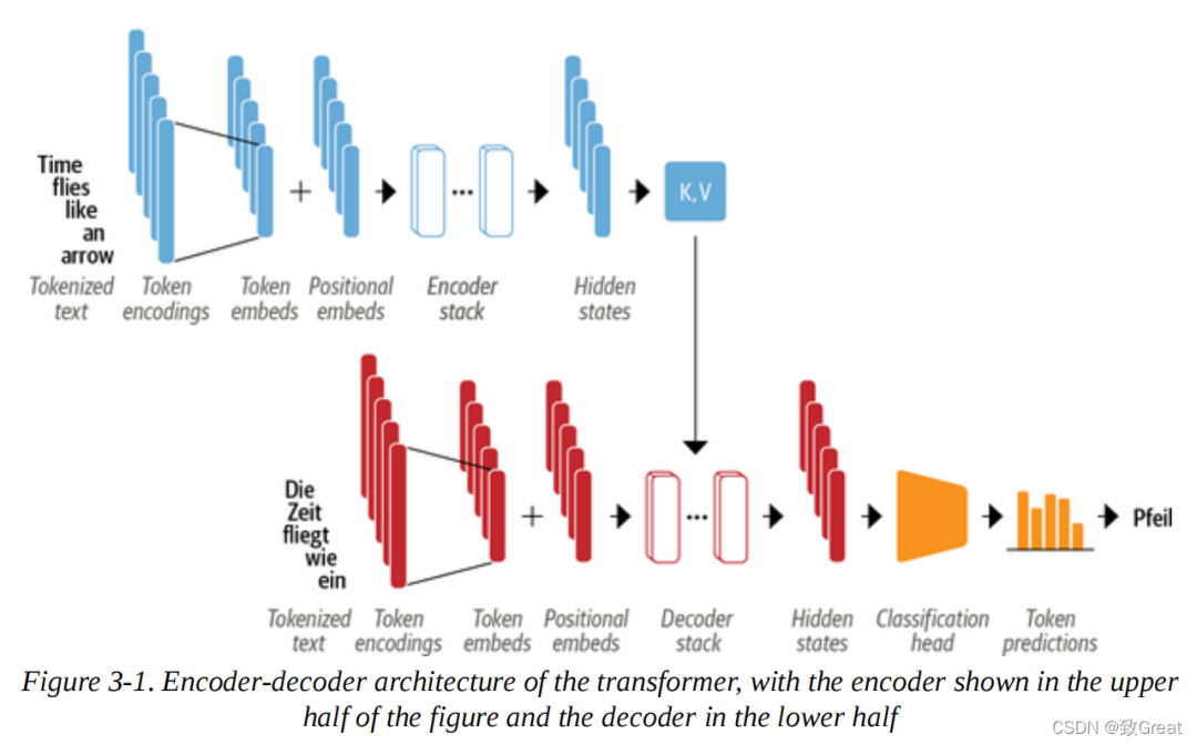
As we saw in Chapter 1, the original Transformer is based on an encoder-decoder architecture, which is widely used for tasks such as machine translation, i.e., translating a string of words from one language to another. This architecture consists of two parts:

Encoder

Transforms the input sequence of tokens into a sequence of embedding vectors, commonly referred to as hidden states or context.

Decoder

Uses the hidden states of the encoder to iteratively generate an output sequence of tokens, one token at a time.

As shown in Figure 3-1, both the encoder and decoder are composed of several components:

We will soon see the details of each component, but we can already see some things that describe the Transformer architecture in Figure 3-1:

The Transformers architecture was initially designed for sequence-to-sequence tasks (like machine translation), but the encoder and decoder modules were quickly adapted into standalone models. Although there are hundreds of different Transformer models, most belong to one of three types:

Pure Encoder These models transform the input text sequence into rich numerical representations, making them well-suited for tasks like text classification or named entity recognition. BERT and its variants, such as RoBERTa and DistilBERT, belong to this class of architectures. In this architecture, the representation computed for a given token depends on both the left (preceding tokens) and the right (subsequent tokens) context. This is often referred to as bidirectional attention.

Pure Decoder Given a text prompt like “Thank you for lunch, I have a…” these models will auto-complete the sequence by iteratively predicting the most likely next word. The GPT family of models falls into this category. In this structure, the representation computed for a given token only depends on the context to its left. This is often referred to as causal or autoregressive attention. Encoder-Decoder These are used to model complex mappings from one text sequence to another; they are suitable for tasks like machine translation and summarization. Besides the Transformer architecture that combines both encoders and decoders that we have already seen, the BART and T5 models also belong to this class.

Considerations

In practice, the application distinctions between pure decoder and pure encoder architectures can be somewhat blurry. For example, pure decoder models like those in the GPT series can be used for tasks like translation, which are typically considered sequence-to-sequence tasks. Similarly, pure encoder models like BERT can be applied to summarization tasks that are usually associated with encoder-decoder or pure decoder models.

Now that you have a high-level understanding of the Transformer architecture, let’s take a closer look at the inner workings of the encoder.

Encoder

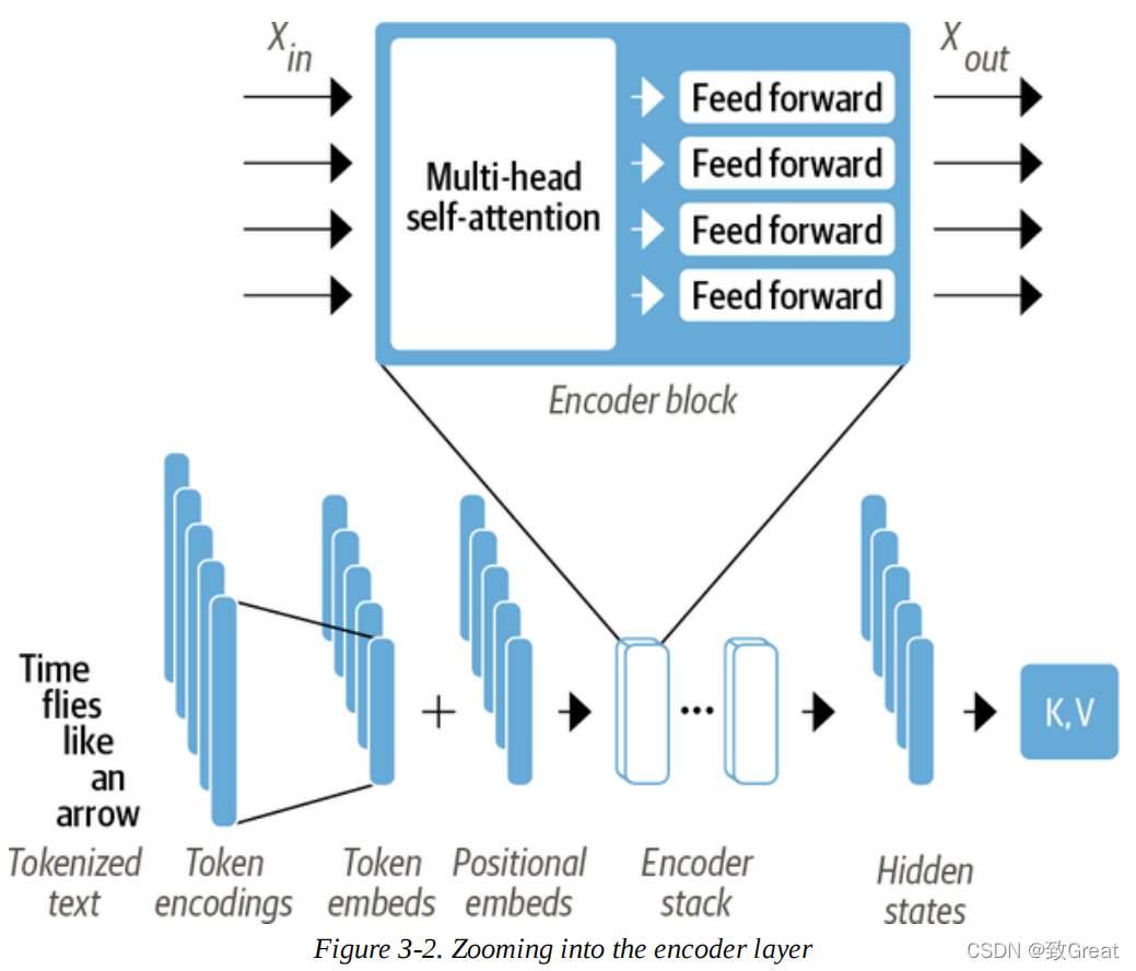
As we saw earlier, the encoder of Transformers consists of many stacked encoder layers. As shown in Figure 3-2, each encoder layer receives a sequence of embedding information and passes it through the following sublayers:

The output embedding of each encoder layer has the same size as the input, and we will soon see that the main function of the encoder stack is to “update” the input embeddings to produce representations that capture some contextual information in the encoded sequence. For example, if “keynote” or “phone” is close to the word “apple”, it will be updated to be more like “company” rather than “fruit”.

Each of these sublayers also uses residual connections and normalization layers, which are standard techniques for effectively training deep neural networks. But to truly understand what makes Transformers work, we need to dive deeper. Let’s start with the most important building block: the self-attention layer.

Self-Attention Layer

Self-Attention Layer

As we discussed in Chapter 1, attention is a mechanism that allows neural networks to assign different weights or “attention” to each element in a sequence. For text sequences, these elements are the token embeddings we encountered in Chapter 2, where each token is mapped to a vector of a fixed dimension. For example, in BERT, each token is represented as a 768-dimensional vector. The “self” part of self-attention refers to the fact that these weights are calculated for all hidden states within the same set – for example, all hidden states of the encoder. In contrast, the attention mechanism associated with recurrent models involves calculating the relevance of each encoder hidden state to the decoder hidden state at a specific decoding time step.

The main idea of self-attention is that we can use the entire sequence to compute a weighted average of each token embedding instead of using fixed embeddings for each token. Another way to phrase this is that given a series of token embeddings, self-attention produces a series of new embeddings, each of which is a linear combination of all: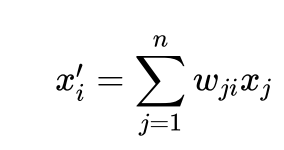

The coefficients are called attention weights and are normalized to ensure.

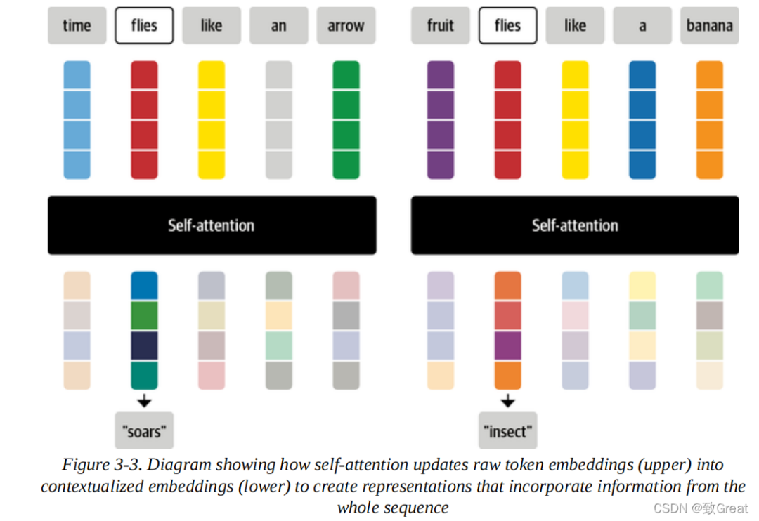
To understand why averaging token embeddings might be a good idea, consider what comes to mind when you see the word “fly”. You might think of the annoying insect, but if given more context, such as “Time flies like an arrow”, you would realize that “flies” refers to a verb. Similarly, we can create a “fly” representation that contains this context by combining all the token embeddings in different proportions, perhaps giving more weight to the embeddings for the words “time” and “arrow”. The embeddings produced in this way are called contextualized embeddings and predate the invention of Transformers in language models like ELMo. Figure 3-3 is a schematic illustration of how two different representations of “fly” are produced through self-attention based on context.

Now let’s see how to calculate the attention weights.

We can visualize how attention weights are calculated using a library called BertViz. This library provides several functions to visualize different aspects of attention in Transformers models. To visualize the attention weights, we can use the neuron_view module of BertViz, which tracks the computation of the weights, to show how the query and key vectors are combined to produce the final weights. Note that you need to click the left “+” to activate the attention visualization:

from transformers import AutoTokenizer 
from bertviz.transformers_neuron_view import BertModel 
from bertviz.neuron_view import show 
model_ckpt = "bert-base-uncased" tokenizer = AutoTokenizer.from_pretrained(model_ckpt)
model = BertModel.from_pretrained(model_ckpt) 
text = "time flies like an arrow" 
show(model, "bert", tokenizer, text, display_mode="light", layer=0, head=8)

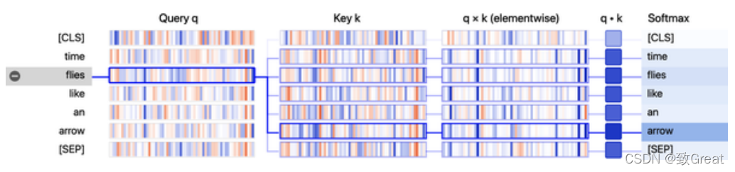
From the visualization, we can see that the values of the query and key vectors are represented as vertical strips, with the intensity of each strip corresponding to the magnitude. The connecting lines are weighted according to the strength of attention between tokens, and we can see that the query vector for “fly” has the strongest overlap with the key vector for “arrow”.

Unveiling the Mystique of Query, Key, and Value The concepts of query, key, and value vectors may seem a bit mysterious when you first encounter them. Their names are inspired by information retrieval systems, but we can use a simple analogy to explain their significance. Imagine you are at the supermarket buying all the ingredients for dinner. You have the recipe for the dish, and each required ingredient can be thought of as a query. As you scan the shelves, you look at the labels (keys) and check if they match the ingredients on your list (similarity function). If there is a match, you take that item off the shelf (value). In this analogy, each matching label allows you to get just one item from the grocery store. Self-attention is a more abstract and “smooth” version: every label in the supermarket matches an ingredient, resulting in every key matching a query. Therefore, if your list includes a dozen eggs, you might end up grabbing 10 eggs, one omelet, and one chicken wing.

Let’s take a closer look at this process by implementing the operation graph for calculating scaled dot-product attention, as shown in Figure 3-4.

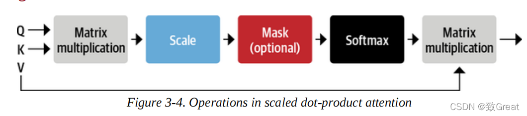
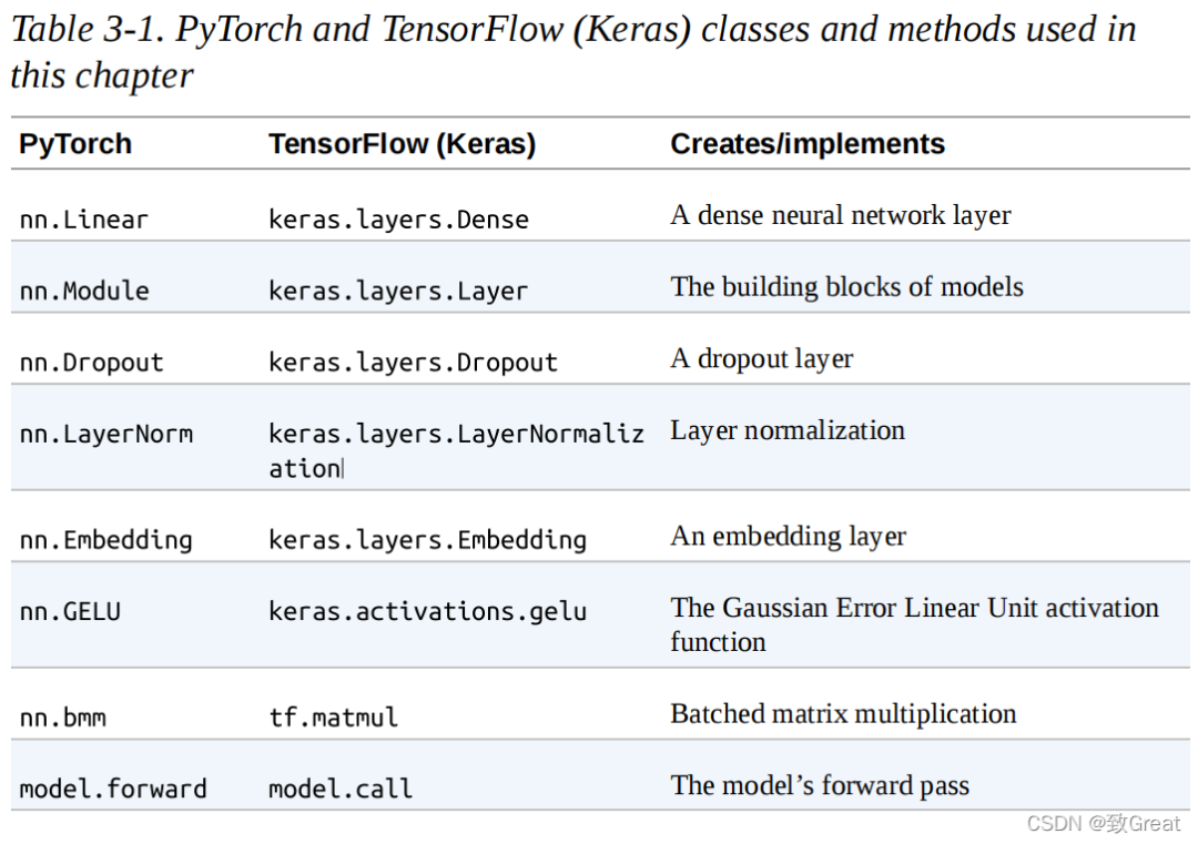
We will use PyTorch to implement the Transformer architecture in this chapter, but the steps in TensorFlow are similar. We provide a mapping of the most important functions between these two frameworks in Table 3-1.

The first thing we need to do is tokenize the text, so let’s use our tokenizer to extract the input IDs:

inputs = tokenizer(text, return_tensors="pt", add_special_tokens=False) 
inputs.input_ids tensor([[ 2051, 10029, 2066, 2019, 8612]])

As we saw in Chapter 2, each token in the sentence is mapped to a unique ID in the tokenizer’s vocabulary. To keep it simple, we also excluded the [CLS] and [SEP] tokens by setting add_special_tokens=False. Next, we need to create some dense embeddings. Here, density means that every entry in the embedding has a non-zero value. In contrast, the one-hot encoding we saw in Chapter 2 is sparse because all entries are zero except for one. In PyTorch, we can do this by using the torch.nn.Embedding layer, which serves as a lookup table for each input ID:

from torch import nn 
from transformers import AutoConfig 
config = AutoConfig.from_pretrained(model_ckpt) 
token_emb = nn.Embedding(config.vocab_size, config.hidden_size) 
token_emb Embedding(30522, 768)

Here, we use the AutoConfig class to load the config.json file associated with the bert-base-uncased model. In Transformers, each model is assigned a configuration file that specifies various hyperparameters, such as vocab_size and hidden_size; in our case, it tells us that each input ID will be mapped to one of the 30,522 embedding vectors stored in nn.Embedding, each of size 768. The AutoConfig class also stores additional metadata, such as label names, for formatting the model’s predictions.

Note at this point that the token embeddings are independent of their context. This means that homonyms (words that are spelled the same but have different meanings), like “fly” in the earlier example, have the same representation. The subsequent attention layer will serve to mix these token embeddings to disambiguate and connect each token’s representation with its contextual content.

Now that we have the lookup table, we can generate embeddings using the input IDs:

inputs_embeds = token_emb(inputs.input_ids) 
inputs_embeds.size() 
torch.Size([1, 5, 768])

This gives us a tensor of shape [batch_size, seq_len, hidden_dim], just like we saw in Chapter 2. We will defer position encoding for now, so the next step is to create the query, key, and value vectors, and use dot product as the similarity function to calculate the attention scores:

import torch from math 
import sqrt 
query = key = value = inputs_embeds 
dim_k = key.size(-1) 
scores = torch.bmm(query, key.transpose(1,2)) / sqrt(dim_k) 
scores.size() 
torch.Size([1, 5, 5])

This creates a 5×5 attention score matrix for each sample in the batch. We will see later that the query, key, and value vectors are produced by independent weight matrices WQ, K, and V applied to the embeddings, but for simplicity, we keep them equal for now. In scaled dot-product attention, the dot product is scaled by the size of the embedding vectors so that we do not get too many large numbers during training, which would cause the softmax we apply next to saturate.

Considerations

The torch.bmm() function performs a batch matrix-matrix multiplication, simplifying the calculation of attention scores, where the query and key vectors have the shape [batch_size, seq_len, hidden_dim]. If we ignore the batch dimension, we could compute the dot product between each query and key vector simply by transposing the key tensor to have the shape [hidden_dim, seq_len] and then using matrix multiplication to collect all the dot products in a [seq_len, seq_len] matrix. Since we want to do this independently for all sequences in the batch, we use torch.bmm(), which requires two batches of matrices and multiplies each matrix in the first batch with the corresponding matrix in the second batch.

Now let’s apply softmax:

import torch.nn.functional as F 
weights = F.softmax(scores, dim=-1) 
weights.sum(dim=-1) 
tensor([[1., 1., 1., 1., 1.]], grad_fn=<SumBackward1>)

The final step is to multiply the attention weights by the value vectors:

attn_outputs = torch.bmm(weights, value) 
attn_outputs.shape torch.Size([1, 5, 768])

And there we have it, we have completed all the steps to implement a simplified form of self-attention! Note that the entire process consists of just two matrix multiplications and one softmax, so you can think of “self-attention” as a fancy form of averaging.

Let’s wrap these steps into a function we can use later:

def scaled_dot_product_attention(query, key, value): 
 dim_k = query.size(-1) 
 scores = torch.bmm(query, key.transpose(1, 2)) / sqrt(dim_k)
 weights = F.softmax(scores, dim=-1) 
 return torch.bmm(weights, value)

Our attention mechanism, when the query and key vectors are equal, will assign a very high score to the same word in the context, especially to the current word itself: the dot product of a query with itself is always 1. However, in practice, the meaning of a word is better defined by complementary words in the context rather than the same word – for example, the meaning of “fly” is better defined by incorporating information from “time” and “arrow” than by mentioning “fly” again. How can we promote this behavior?

Let’s allow the model to project our initial token vectors into three different spaces using three different linear projections to create a set of distinct vectors for queries, keys, and values.

Multi-Head Attention

In our simple example, we were just using the embeddings “as is” to calculate attention scores and weights, but that is far from the whole story. In practice, the self-attention layer applies three independent linear transformations to each embedding to produce the query, key, and value vectors. These transformations project the embeddings, each with its own set of learnable parameters, allowing the self-attention layer to focus on different semantic aspects of the sequence.

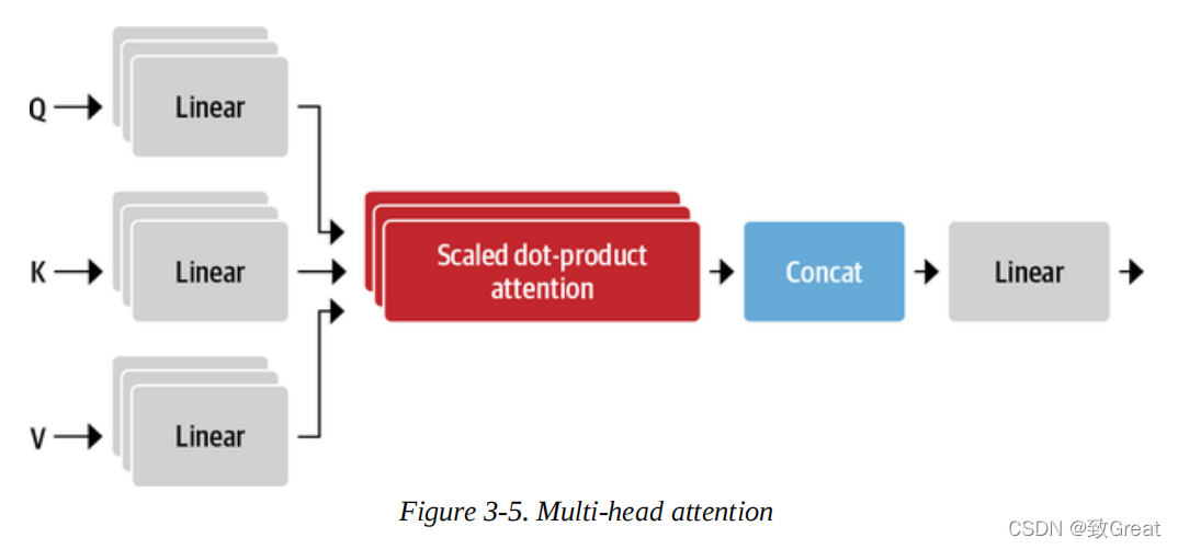
It turns out that having multiple sets of linear projections is also beneficial, with each set representing what is called an attention head. The resulting multi-head attention layer is illustrated in Figure 3-5. But why do we need more than one attention head? The reason is that the softmax of one head often focuses primarily on one aspect of similarity. With several heads, the model can attend to multiple aspects simultaneously. For example, one head might focus on the interaction between the subject and the verb, while another head finds nearby adjectives. Clearly, we are not hand-crafting these relationships into the model; they are learned entirely from the data. If you are familiar with computer vision models, you might find it similar to filters in convolutional neural networks, where one filter is responsible for detecting faces, and another looks for the wheels of cars in images.

Let’s implement this layer, starting by encoding a single attention head:

class AttentionHead(nn.Module): 
 def __init__(self, embed_dim, head_dim): 
        super().__init__() 
        self.q = nn.Linear(embed_dim, head_dim) 
        self.k = nn.Linear(embed_dim, head_dim) 
        self.v = nn.Linear(embed_dim, head_dim) 
 def forward(self, hidden_state): 
  attn_outputs = scaled_dot_product_attention( self.q(hidden_state), self.k(hidden_state), self.v(hidden_state)) 
  return attn_outputs

Here, we initialize three independent linear layers that apply matrix multiplication to the embedding vectors, producing tensors of shape [batch_size, seq_len, head_dim], where head_dim is the dimension we are projecting to. While head_dim does not necessarily have to be smaller than the embedding dimension (embed_dim), in practice, it is selected as a multiple of embed_dim so that the computational load per head remains constant. For example, BERT has 12 attention heads, so each head has a size of 768/12=64.

Now that we have an attention head, we can concatenate the outputs of each attention head to implement a complete multi-head attention layer:

class MultiHeadAttention(nn.Module): 
 def __init__(self, config): 
  super().__init__() 
  embed_dim = config.hidden_size 
  num_heads = config.num_attention_heads 
  head_dim = embed_dim // num_heads 
  self.heads = nn.ModuleList( [AttentionHead(embed_dim, head_dim) for _ in range(num_heads)] ) 
  self.output_linear = nn.Linear(embed_dim, embed_dim) 
 def forward(self, hidden_state): 
  x = torch.cat([h(hidden_state) for h in self.heads], dim=-1) 
  x = self.output_linear(x) 
  return x

Note that the concatenated output of the attention heads is also fed into the final linear layer to produce an output tensor of shape [batch_size, seq_len, hidden_dim], suitable for downstream feed-forward networks. To confirm, let’s check if the multi-head attention layer produces the expected shape for our input:

multihead_attn = MultiHeadAttention(config) 
attn_output = multihead_attn(inputs_embeds) 
attn_output.size() 
torch.Size([1, 5, 768] )

It works! To summarize this section on attention, let’s once again use BertViz to visualize the attention of the two different usages of the word “fly”. Here, we can use the head_view() function of BertViz to compute the attention of a pre-trained model and point out the positions of sentence boundaries:

from bertviz import head_view 
from transformers import AutoModel 
model = AutoModel.from_pretrained(model_ckpt, output_attentions=True) 
sentence_a = "time flies like an arrow" 
sentence_b = "fruit flies like a banana" 
viz_inputs = tokenizer(sentence_a, sentence_b, return_tensors='pt') 
attention = model(**viz_inputs).attentions 
sentence_b_start = (viz_inputs.token_type_ids == 0).sum(dim=1) 
tokens = tokenizer.convert_ids_to_tokens(viz_inputs.input_ids[0]) 
head_view(attention, tokens, sentence_b_start, heads=[8])

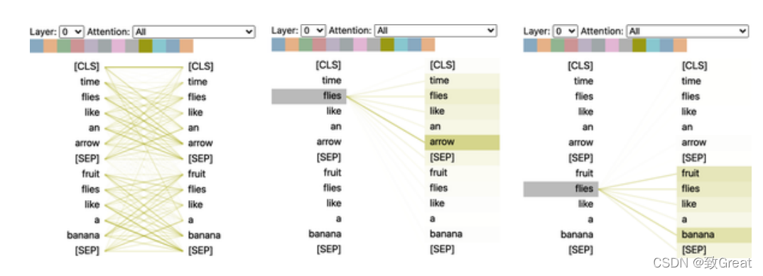
This visualization shows the attention weights, which are the lines connecting the updated tokens (on the left) and each word being attended to (on the right). The strength of the lines indicates the strength of the attention weights, with darker lines representing values close to 1 and lighter lines representing values close to 0. In this example, the input consists of two sentences, and the [CLS] and [SEP] tokens are the special tokens we encountered in the BERT tokenizer in Chapter 2. One thing we can see from the visualization is that the attention weights are strongest between words belonging to the same sentence, indicating that BERT can tell which words to attend to within the same sentence. However, for the word “fly”, we can see that BERT identifies “arrow” as important in the first sentence, while in the second sentence, it identifies “fruit” and “banana” as important. These attention weights allow the model to distinguish between the use of “flies” as a verb or a noun, depending on the context in which it appears!

Now that we have covered attention, let’s take a look at how to implement the remaining part of the encoder layer: the position-wise feed-forward network.

Feed-Forward Layer

The feed-forward sublayers in both the encoder and decoder are simply a simple two-layer fully connected neural network but with a slight difference: it processes each embedding independently instead of treating the entire embedding sequence as a single vector. For this reason, this layer is often referred to as the position-wise feed-forward layer. You might also see it referred to as a 1D convolution with kernel size 1, a term commonly used by those with a computer vision background (for example, OpenAI’s GPT codebase uses this nomenclature). An empirical rule in the literature is that the hidden size of the first layer is four times the embedding size, and the most commonly used activation function is GELU. This is the most memory-intensive part and is the part most often expanded when scaling up the model. We can implement it as a simple nn.Module as follows:

class FeedForward(nn.Module): 
 def __init__(self, config): 
        super().__init__() 
        self.linear_1 = nn.Linear(config.hidden_size, config.intermediate_size) 
        self.linear_2 = nn.Linear(config.intermediate_size, config.hidden_size) 
        self.gelu = nn.GELU() 
        self.dropout = nn.Dropout(config.hidden_dropout_prob) 
 def forward(self, x): 
  x = self.linear_1(x) 
  x = self.gelu(x) 
  x = self.linear_2(x) 
  x = self.dropout(x) 
  return x

Note that feed-forward layers like nn.Linear are typically applied to a tensor of shape (batch_size, input_dim) and operate independently on each element of the batch dimension. In practice, this means that when we pass a tensor of shape (batch_size, seq_len, hidden_dim) through this layer, it applies independently to all token embedding vectors in the batch and input sequence, which is exactly what we want. Let’s test this by passing the attention outputs through it:

feed_forward = FeedForward(config) 
ff_outputs = feed_forward(attn_outputs) 
ff_outputs.size() 
torch.Size([1, 5, 768])

We now have all the components needed to create a mature Transformers encoder layer. The only decision left is where to place the residual connections and normalization layers. Let’s see how this affects the model structure.

Adding Normalization Layer

As mentioned earlier, the Transformer architecture leverages layer normalization and residual connections. The former normalizes each input in the batch to have zero mean and unit variance. The residual connection passes the tensor to the next layer of the model without processing it and adds it to the processed tensor. When it comes to where to place the normalization layer in the encoder or decoder layers of Transformers, there are primarily two choices in the literature:

Post-Layer Normalization This is the arrangement used in the Transformer paper; it places the normalization layer between the residual connections. This arrangement can be tricky for training from scratch as the gradients may become biased. For this reason, you often see a concept called learning rate warm-up, where the learning rate gradually increases from a small value to some maximum value during training. Pre-Layer Normalization This is the most common arrangement found in the literature; it places the normalization layer within the span of the residual connections. This tends to be more stable during training and usually does not require any learning rate warm-up.

Figure 3-6 illustrates the differences between these two arrangements:

We will use the second arrangement, so we can simply glue our blocks together as follows:

class TransformerEncoderLayer(nn.Module): 
 def __init__(self, config): 
        super().__init__() 
        self.layer_norm_1 = nn.LayerNorm(config.hidden_size) 
        self.layer_norm_2 = nn.LayerNorm(config.hidden_size) 
        self.attention = MultiHeadAttention(config) 
        self.feed_forward = FeedForward(config) 
 def forward(self, x): 
  # Apply layer normalization and then copy input into query, key, valu
  hidden_state = self.layer_norm_1(x) 
  # Apply attention with a skip connection 
  x = x + self.attention(hidden_state) 
  # Apply feed-forward layer with a skip connection 
  x = x + self.feed_forward(self.layer_norm_2(x)) 
  return x

Now let’s test this with our input embeddings:

encoder_layer = TransformerEncoderLayer(config) 
inputs_embeds.shape, encoder_layer(inputs_embeds).size() 
(torch.Size([1, 5, 768]), torch.Size([1, 5, 768]))

We have now implemented our first Transformers encoder layer from scratch! However, there is one caveat regarding how we set up the encoder layers: they are completely invariant to the positions of the tokens. Since the multi-head attention layer is essentially a fancy weighted sum, information about the positions of the tokens is lost.

Fortunately, there is a simple trick to incorporate position information using position embeddings. Let’s take a look at this.

Position Embeddings

Position embeddings are based on a simple but very effective idea: to enhance token embeddings with a pattern of values related to the positions arranged in a vector. If the pattern is characteristic for each position, the attention heads and feed-forward layers in each stack can learn to incorporate positional information into their transformations.

There are several ways to implement this, one of the most popular methods is to use learnable patterns, especially when the pre-training dataset is large enough. This works exactly like token embeddings, but uses position indices instead of token IDs as input. By this method, an effective way to encode token positions can be learned during pre-training.

Let’s create a custom embedding module that combines a token embedding layer that projects input_ids into a dense hidden state while also combining position embeddings that do the same for position_ids. The resulting embeddings are a simple sum of the two embeddings:

class Embeddings(nn.Module): 
 def __init__(self, config): 
        super().__init__() 
        self.token_embeddings = nn.Embedding(config.vocab_size, config.hidden_size) 
        self.position_embeddings = nn.Embedding(config.max_position_embeddings, config.hidden_size) 
        self.layer_norm = nn.LayerNorm(config.hidden_size, eps=1e-12) 
        self.dropout = nn.Dropout() 
 def forward(self, input_ids): 
        # Create position IDs for input sequence 
        seq_length = input_ids.size(1) 
        position_ids = torch.arange(seq_length, dtype=torch.long).unsqueeze(0) 
        # Create token and position embeddings 
        token_embeddings = self.token_embeddings(input_ids) 
        position_embeddings = self.position_embeddings(position_ids) 
        # Combine token and position embeddings 
        embeddings = token_embeddings + position_embeddings 
        embeddings = self.layer_norm(embeddings) 
        embeddings = self.dropout(embeddings) 
        return embeddings 
    embedding_layer = Embeddings(config) 
    embedding_layer(inputs.input_ids).size() 
    torch.Size([1, 5, 768])

We see that the embedding layer now creates a single, dense embedding for each token.

While learnable position embeddings are easy to implement and widely used, there are also some alternatives.

Absolute Position Representations

Transformers models can use a static pattern consisting of modulated sine and cosine signals to encode the positions of tokens. This method works particularly well when there is not a lot of data available.

Relative Position Representations

While absolute positions are important, it can be argued that the surrounding tokens are most important when calculating embeddings. Relative position representations follow this intuition and encode the relative positions between tokens. This cannot be established by introducing a new relative embedding layer at the start because each token’s relative embedding will change depending on which position we are attending to in the sequence. Instead, the attention mechanism itself is modified to include terms that account for the relative positions between tokens. Models like DeBERTa use such representations.

Now, let’s put all this together to build a complete Transformers encoder that combines embeddings and encoder layers:

class TransformerEncoder(nn.Module): 
 def __init__(self, config): super().__init__() 
  self.embeddings = Embeddings(config) 
  self.layers = nn.ModuleList([TransformerEncoderLayer(config) for _ in range(config.num_hidden_layers)]) 
 def forward(self, x): x = self.embeddings(x) 
  for layer in self.layers: 
   x = lay 
  return x
  

Let’s check the output shape of the encoder:

encoder = TransformerEncoder(config) 
encoder(inputs.input_ids).size()
torch.Size([1, 5, 768])

We can see that we get a hidden state for each token in the batch. This output format makes the architecture very flexible, allowing us to easily adapt it to various applications, such as predicting missing tokens in masked language modeling or predicting the start and end positions of answers in question answering. In the next section, we will see how to build a classifier like the one we used in Chapter 2.

Adding a Classification Head

Transformers models are typically divided into a task-independent body and a task-specific head. We will encounter this pattern again when we look at design patterns for Transformers in Chapter 4. So far, what we have built is the body, so if we want to build a text classifier, we need to attach a classification head to this body. We have a hidden state for each token, but we only need to make one prediction. There are several schemes to handle this problem. Traditionally, the first token in such models is used for prediction, and we can attach a dropout and a linear layer for classification prediction. The class below extends the existing encoder for sequence classification:

class TransformerForSequenceClassification(nn.Module): 
 def __init__(self, config): 
  super().__init__() 
  self.encoder = TransformerEncoder(config) 
  self.dropout = nn.Dropout(config.hidden_dropout_prob) 
  self.classifier = nn.Linear(config.hidden_size, config.num_labels) 
 def forward(self, x): 
  x = self.encoder(x)[:, 0, :] 
  # select hidden state of [CLS] token 
  x = self.dropout(x) 
  x = self.classifier(x) 
  return x

Before initializing the model, we need to define how many classes we want to predict:

config.num_labels = 3 
encoder_classifier = TransformerForSequenceClassification(config) 
encoder_classifier(inputs.input_ids).size() 

torch.Size([1, 3])

This is exactly what we were looking for. For each example in the batch, we got the unnormalized logits for each class in the output.

This concludes our analysis of the encoder and how we can combine it with a task-specific head. Now let’s turn our attention to the decoder.

Decoder

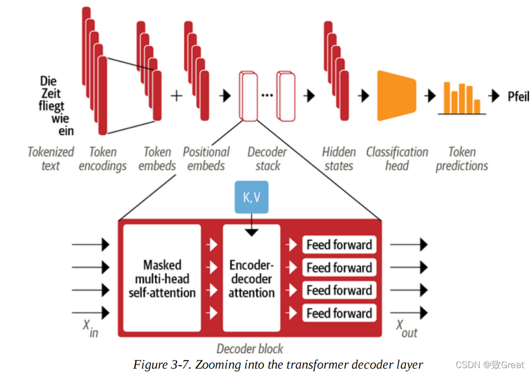
As shown in Figure 3-7, the main difference between the decoder and the encoder is that the decoder has two attention sublayers:

Masked Multi-Head Self-Attention Layer Ensures that the tokens generated at each time point are based only on past outputs and the currently predicted token. Without this, the decoder could cheat during training by simply copying the target translation; masking the input ensures that this task is not trivial. Encoder-Decoder Attention Layer Performs multi-head attention on the output keys and values from the encoder stack, with the intermediate representation of the decoder serving as the query. This way, the encoder-decoder attention layer learns how to relate tokens from two different sequences, such as two different languages. The decoder has access to the encoder’s keys and values in each block.

Let’s take a look at the modifications we need to make to include masking in our self-attention layer and consider the implementation of the encoder-decoder attention layer as a homework problem. The trick for masked self-attention is to introduce a mask matrix, which has 1s below the diagonal and 0s above:

seq_len = inputs.input_ids.size(-1) 
mask = torch.tril(torch.ones(seq_len, seq_len)).unsqueeze(0) 
mask[0]

tensor([
[1., 0., 0., 0., 0.], 
[1., 1., 0., 0., 0.], 
[1., 1., 1., 0., 0.], 
[1., 1., 1., 1., 0.], 
[1., 1., 1., 1., 1.]
])

Here we used PyTorch’s tril() function to create a lower triangular matrix. Once we have this mask matrix, we can prevent each attention head from peeking at future tokens by replacing all the 0s with negative infinity using Tensor.masked_fill():

scores.masked_fill(mask == 0, -float("inf")) 

tensor([[
[26.8082, -inf, -inf, -inf, -inf], 
[-0.6981, 26.9043, -inf, -inf, -inf], 
[-2.3190, 1.2928, 27.8710, -inf, -inf], 
[-0.5897, 0.3497, -0.3807, 27.5488, -inf], 
[ 0.5275, 2.0493, -0.4869, 1.6100, 29.0893]]], grad_fn=<MaskedFillBackward0>)

By setting the upper limit to negative infinity, we ensure that once we take the softmax of the scores, the attention weights are all zero, because e-∞=0 (remember that softmax computes normalized exponentials). We can easily include this masking behavior by making a small modification to the scaled dot-product attention function we implemented earlier:

def scaled_dot_product_attention(query, key, value, mask=None): 
 dim_k = query.size(-1) 
 scores = torch.bmm(query, key.transpose(1, 2)) / sqrt(dim_k) 
 if mask is not None: 
  scores = scores.masked_fill(mask == 0, float("-inf")) 
 weights = F.softmax(scores, dim=-1) 
 return weights.bmm(value)

From here, building the decoding layer is quite straightforward; we point the reader to Andrej Karpathy’s excellent implementation of minGPT for the details.

We have given you a lot of technical information here, but now you should have a good understanding of each block of the Transformer architecture. Before we proceed to build models for more advanced tasks than text classification, let’s take a step back and look at the situation of different Transformer models and their relationships to complete this chapter.

Unveiling the Mystique of Encoder-Decoder Attention

Let’s see if we can shed some light on the mysteries of encoder-decoder attention. Imagine you (the decoder) are taking an exam in class. Your task is to predict the next word based on the previous words (decoder input), which sounds simple but is very difficult (try predicting the next word of a passage in this book yourself). Luckily, your neighbor (the encoder) has the complete text. Unfortunately, they are a foreign exchange student, and the text is in their native language. Clever students, you still figure out a way to cheat. You draw a little cartoon illustrating the text you have (Query) and give it to your neighbor. They try to find a paragraph that matches that description (Key), draw a cartoon of the words that follow that paragraph (Value), and then send it back to you. With this system, you can win the exam.

Understanding Transformers

As you have seen in this chapter, there are three main architectures of Transformers models: encoder, decoder, and encoder-decoder. The initial success of early Transformers models sparked a Cambrian explosion of model development, as researchers built models on datasets of different scales and natures, using new pre-training objectives, and adjusting architectures to further improve performance. Although the zoo of models continues to grow rapidly, they can still be categorized into these three types.

In this section, we will provide a brief introduction to the most important Transformers models in each class. Let’s first take a look at the family tree of Transformers.

Transformers Family

Over time, each of the three main architectures has undergone its own evolution. Figure 3-8 illustrates this, showing several of the most prominent models and their descendants.

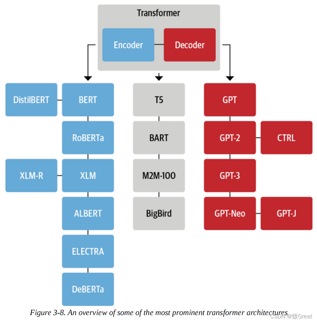
There are over 50 different architectures included in Transformers, and this family tree is by no means a complete overview of all existing architectures; it merely highlights some milestone architectures. We have delved deeply into the original Transformer architecture in this chapter, so let’s take a closer look at some key evolutions, starting with the encoder branch.

Encoder Branch

The first pure encoder model based on the Transformer architecture is BERT. When it was published, it outperformed all state-of-the-art models on the popular GLUE benchmark, which measures natural language understanding (NLU) across several tasks of varying difficulty. Subsequently, BERT’s pre-training objectives and architecture were adjusted to further improve performance. In NLU tasks such as text classification, named entity recognition, and question answering, encoder-only models still dominate in research and industry. Let’s briefly understand the BERT model and its variants. BERT BERT’s pre-training has two objectives: predicting masked tokens in the text and determining whether one text segment may follow another. The former task is called masked language modeling (MLM), and the latter is called next sentence prediction (NSP). DistilBERT

While BERT provides good results, its size can make it cumbersome to deploy in low-latency environments. By using a technique called knowledge distillation during pre-training, DistilBERT achieves 97% of BERT’s performance while reducing memory usage by 40% and speeding up by 60%. You can find more details about knowledge distillation in Chapter 8.

RoBERTa

A study conducted after BERT’s release showed that modifying the pre-training scheme could further improve its performance. RoBERTa was trained for longer, on larger batches with more training data, and it abandoned the NSP task. These changes combined significantly improved its performance compared to the original BERT model. XLM

The work on cross-lingual language models (XLM) explored several pre-training objectives for building multilingual models, including autoregressive language modeling from GPT-like models and MLM from BERT. Additionally, the authors of the paper on XLM pre-training introduced translation language modeling (TLM), an extension of MLM for multilingual input. By experimenting with these pre-training tasks, they achieved state-of-the-art results on several multilingual NLU benchmarks as well as translation tasks. XLM-RoBERTa

Following the work on XLM and RoBERTa, XLM-RoBERTa or XLM-R model advanced multilingual pre-training by massively scaling up the training data. Utilizing the Common Crawl corpus, its developers created a dataset with 2.5TB of text; then they trained an encoder on this dataset using MLM. Since this dataset only contains non-parallel text (i.e., translations), the TLM objective of XLM was abandoned. This approach largely outperformed both XLM and multilingual BERT variants, especially on low-resource languages.

ALBERT

The ALBERT model introduces three changes to make the encoder’s structure more efficient. First, it decouples the token embedding dimension from the hidden dimension, allowing for a smaller embedding dimension, which saves parameters, especially as the vocabulary size increases. Second, all layers share the same parameters, further reducing the number of effective parameters. Finally, the NSP objective is replaced with sentence ordering prediction: the model needs to predict whether two consecutive sentences are swapped, rather than predicting whether they belong together at all. These changes make it possible to train larger models with fewer parameters and achieve outstanding performance on NLU tasks. ELECTRA

A limitation of the standard MLM pre-training objective is that only the representations of masked tokens are updated at each training step, while other input tokens are not updated. To address this, ELECTRA uses a dual model approach: the first model (usually small) works like a standard masked language model and predicts masked tokens. The second model, called the discriminator, then has the task of predicting which tokens in the output of the first model were originally masked. Thus, the discriminator needs to perform binary classification for each token, resulting in a 30-fold increase in training efficiency. For downstream tasks, the discriminator is fine-tuned like a standard BERT model.

DeBERTa

The DeBERTa model introduces two architectural changes. First, each token is represented as two vectors: one representing content and the other representing relative position. By separating the content of the tokens from their relative positions, the self-attention layer can better model the dependencies between nearby tokens. On the other hand, the absolute position of a word is also important, especially for decoding. For this reason, an absolute position embedding is added before the softmax layer of the token decoding head. DeBERTa is the first model to surpass human baselines (as a combination) on the SuperGLUE benchmark, which is a more difficult version of GLUE consisting of several sub-tasks for measuring NLU performance.

Now that we have highlighted some of the major pure encoder architectures, let’s take a look at the pure decoder models.

Decoder Branch

Advancements in Transformers decoder models have largely been led by OpenAI. These models excel at predicting the next word in a sequence, making them primarily used for text generation tasks (detailed in Chapter 5). Their advancements have been propelled by using larger datasets and scaling language models to larger sizes. Let’s take a look at the evolution of these fascinating generative models. GPT

The introduction of GPT combined two key ideas in NLP: a novel and efficient Transformers decoder architecture and transfer learning. In that setup, the model is pre-trained by predicting the next word based on previous words. The model was trained on BookCorpus and achieved tremendous results on downstream tasks such as classification. GPT-2

Inspired by the success of the simple and scalable pre-training method, the original model and training set were scaled up to produce GPT-2. This model is capable of generating coherent text over long sequences. Due to concerns about potential misuse, the model was released in a phased manner, with smaller models released first and the full model released later. CTRL

Models like GPT-2 can continue an input sequence (also called a prompt). However, users have almost no control over the style of the generated sequences. The Conditional Transformers Language (CTRL) model addresses this issue by adding “control tokens” at the beginning of the sequence. These allow for controlling the style of generated text, enabling diverse generation.

GPT-3

After successfully scaling GPT to GPT-2, a thorough analysis of the behavior of language models of different scales revealed a simple power-law relationship between compute, dataset size, model size, and the performance of language models. Inspired by these insights, GPT-2 was scaled up 100 times to produce GPT-3, which has 175 billion parameters. Besides being able to generate impressive realistic text paragraphs, this model also exhibits few-shot learning capabilities: with just a few examples of new tasks, such as translating text into code, the model can perform the task on new examples. OpenAI has not open-sourced this model but provides an interface through OpenAI’s API.

GPT-Neo/GPT-J-6B

GPT-Neo and GPT-J-6B are GPT-like models trained by EleutherAI, a collective of researchers aiming to recreate and release models of GPT-3 scale. The current models are smaller variants of the full 175 billion parameter model, with 1.3 billion, 2.7 billion, and 6 billion parameters, competing with the smaller GPT-3 models provided by OpenAI.

The final branch of the Transformers family tree is the encoder-decoder models. Let’s take a look.

Encoder-Decoder Branch

While it has been common to build models using a single encoder or decoder stack, the Transformer architecture has several encoder-decoder variants that have new applications in both NLU and NLG:

T5

The T5 model unifies all NLU and NLG tasks by converting them into text-to-text tasks. All tasks are set as sequence-to-sequence tasks, where adopting the encoder-decoder architecture is quite natural. For example, for a text classification problem, this means that the text is used as input to the encoder, while the decoder must generate the label as normal text rather than a category. We will explore this in more detail in Chapter 6. The T5 architecture uses the original Transformer architecture. Pre-trained on a large scraped dataset called C4, the model was trained with masked language modeling and SuperGLUE tasks by converting all tasks into text-to-text tasks. The largest model with 11 billion parameters achieved state-of-the-art results on several benchmarks.

BART

BART combines the pre-training procedures of BERT and GPT in an encoder-decoder architecture. Input sequences undergo several possible transformations, from simple masking to sentence shuffling, token deletion, and document rotation. These modified inputs pass through the encoder, while the decoder must reconstruct the original text. This makes the model more flexible, as it can potentially be used for both NLU and NLG tasks, achieving state-of-the-art performance in both.

M2M-100

Traditionally, a translation model is built for a specific language pair and translation direction. However, this does not scale to many languages, and there may be shared knowledge between language pairs that can be leveraged for translations between low-resource languages. M2M-100 is the first translation model that can translate between any of 100 languages. This allows for high-quality translations between rare and underrepresented languages. The model uses prefix tokens (similar to special [CLS] tokens) to indicate the source and target languages.

BigBird

A major limitation of Transformers models is the maximum context size due to the quadratic memory requirements of the attention mechanism. BigBird addresses this by using a sparsely formed attention with linear scaling. This allows the context size to be dramatically expanded from 512 tokens in most BERT models to 4096 tokens in BigBird. This is particularly useful in cases where long dependencies need to be preserved, such as in text summarization.

All pre-trained models from the models we saw in this section can be found on the Hugging Face Hub and can be fine-tuned for your use case using Transformers, as discussed in the previous chapter.

Summary

In this chapter, we started with the core of the Transformer architecture, delving into the self-attention mechanism, and then added all the necessary parts to build a Transformer encoder model.

We added embedding layers for tokens and positional information, built a feed-forward layer to complement the attention heads, and finally added a classification head on top of the model body for predictions. We also looked at the decoder aspects of the Transformer architecture and summarized the most important model architectures at the end of this chapter. Now that you have a better understanding of the fundamentals, let’s move beyond simple classification and build a multilingual named entity recognition model.