Star ★TopPublic AccountLove you all♥
Author: Nayak Translated by: 1+1=6
0
Introduction
This article is based on a research paper titled“Algorithmic Financial Trading with Deep Convolutional Neural Networks: Time Series to Image Conversion Approach”:
Get the paper at the end of the article
We borrowed some core ideas from the authors of this paper while making some improvements.
Get related code at the end of the article
1
What does the paper say?
In this section, we will explain the points raised in the paper:
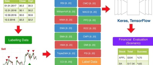
Calculate 15 technical indicators in your trading data, with 15 different period lengths each day. Then convert the 225 (15*15) new features into 15*15 images. Label the data as buy/sell/hold according to the algorithms provided in the paper. Then train a convolutional neural network classifier like any other image classification problem.
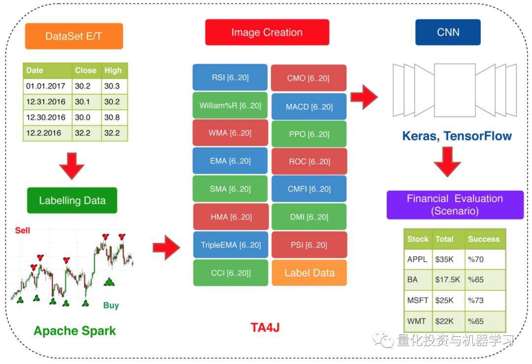
Image from: the paper
We use the Simple Moving Average (SMA) to explain the concept of technical indicators and periods:
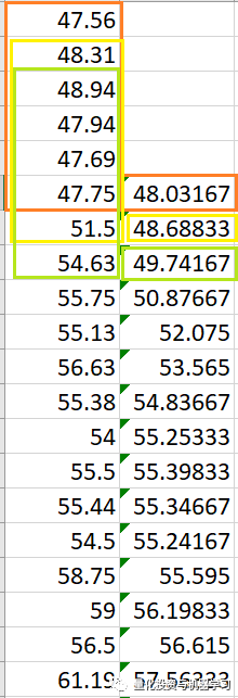
6-day rolling
Now each row in the dataset has 15 new features. If these numbers are recombined into a 15×15 array, an image is obtained! But one thing to keep in mind is to maintain the spatial proximity of the relevant technical indicators when constructing these images. You should know that when training a face recognition model, if there is an eye below a nose in a picture, you definitely wouldn’t label it as a face.
1. Labeling
The authors used the following algorithm:
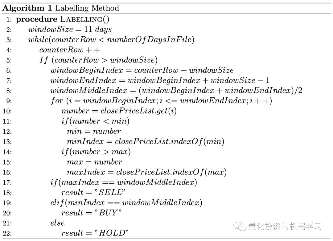
Image from: the paper
Utilizing the closing price within an 11-day window. If the middle number in the window is the largest, the last day (the 11th day) is labeled as “sell”; if the middle number is the smallest, the last day is labeled as “buy”; otherwise, it is labeled as “hold”. Slide the window and repeat as explained earlier. The idea is to buy at the bottom and sell at the peak of any 11-day window.
2. Training
The authors used a rolling window for training. Suppose our historical data is from 2000 to 2019, train with 5 years of data, and test with 1 year of data. This means extracting data from 2000 – 2004 for training and using 2005 data for testing. Train and test your model based on this data. And so on, as shown in the figure below:
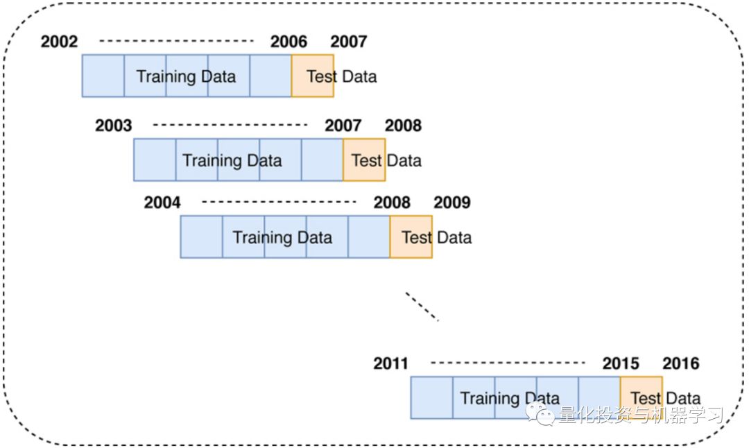
Image from: the paper
3. Model Performance Evaluation
The authors provided two types of model evaluation in the paper: computational performance evaluation and financial performance evaluation. Computational performance evaluation includes confusion matrix, F1 score, class accuracy, etc. Financial performance evaluation is done by applying the model predictions in a real trading environment and considering returns. Here, we will consider computational performance evaluation.
2
Model Implementation
As mentioned at the beginning of this article, we did not strictly follow the research paper, as it did not yield the expected results. We made some modifications, and the results are on par with the paper, and in some cases even better.
1. Data
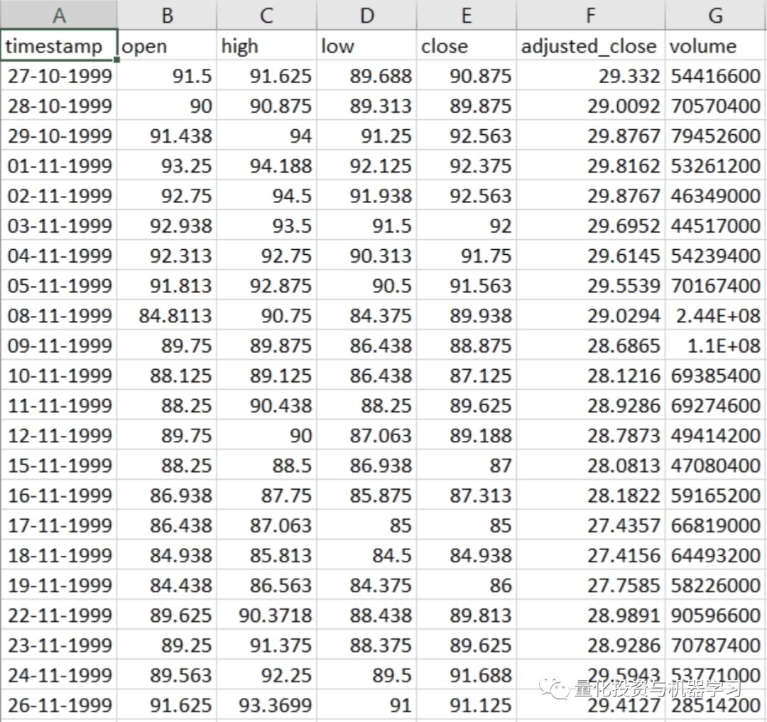
If you want to study US stock data domestically, WindQuant (www.windquant.com) can be used:
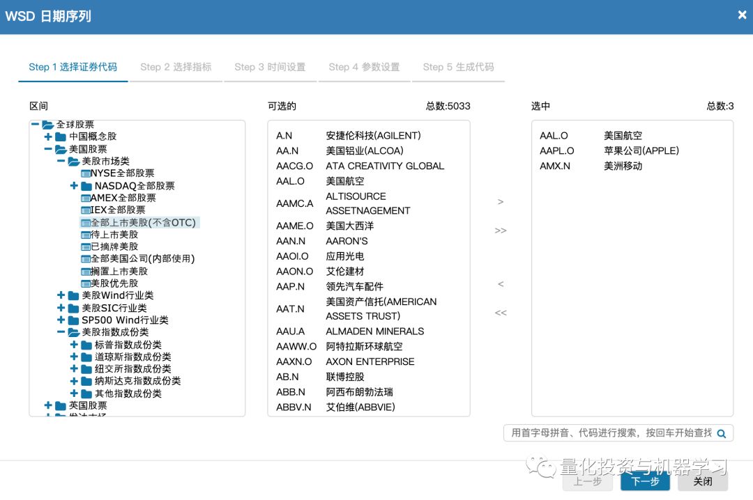
Image from: www.windquant.com
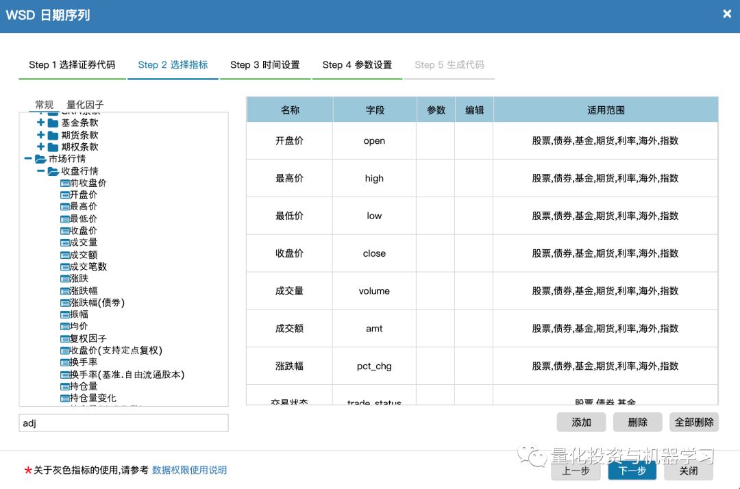
Image from: www.windquant.com
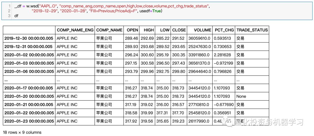
Image from: www.windquant.com
2. Feature Engineering
We used some of the indicators from the paper (the first deviation), and all indicator codes are in the utils.py file.
Get related code at the end of the article
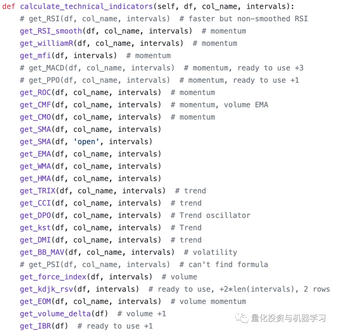

Image from: code file
WindQuant (www.windquant.com) also provides direct functions to calculate technical indicators, just call them directly, and parameters can also be adjusted:
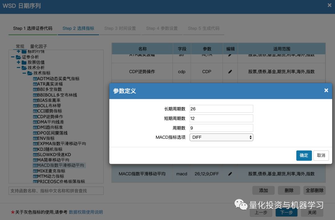
Image from: www.windquant.com
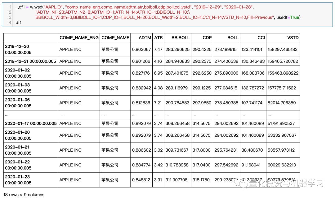
Image from: www.windquant.com
3. Labeling Data
In this article, we used the original labeling algorithm from the authors. Code implementation:
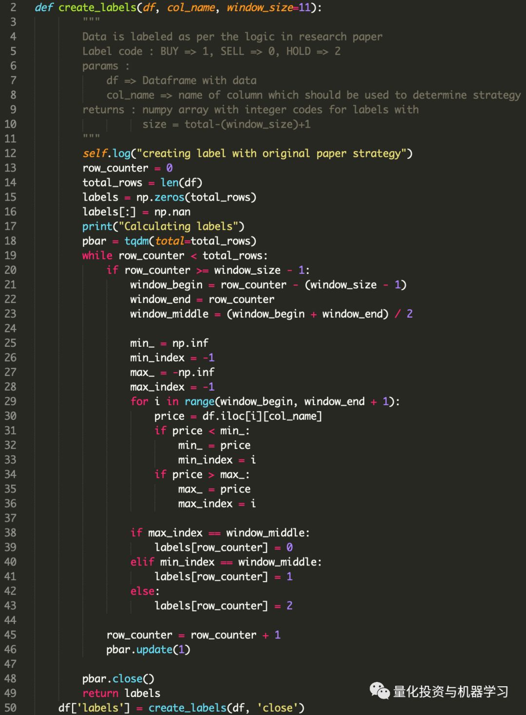
Dataset after labeling:
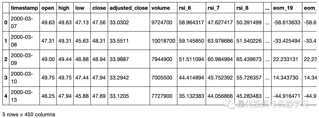
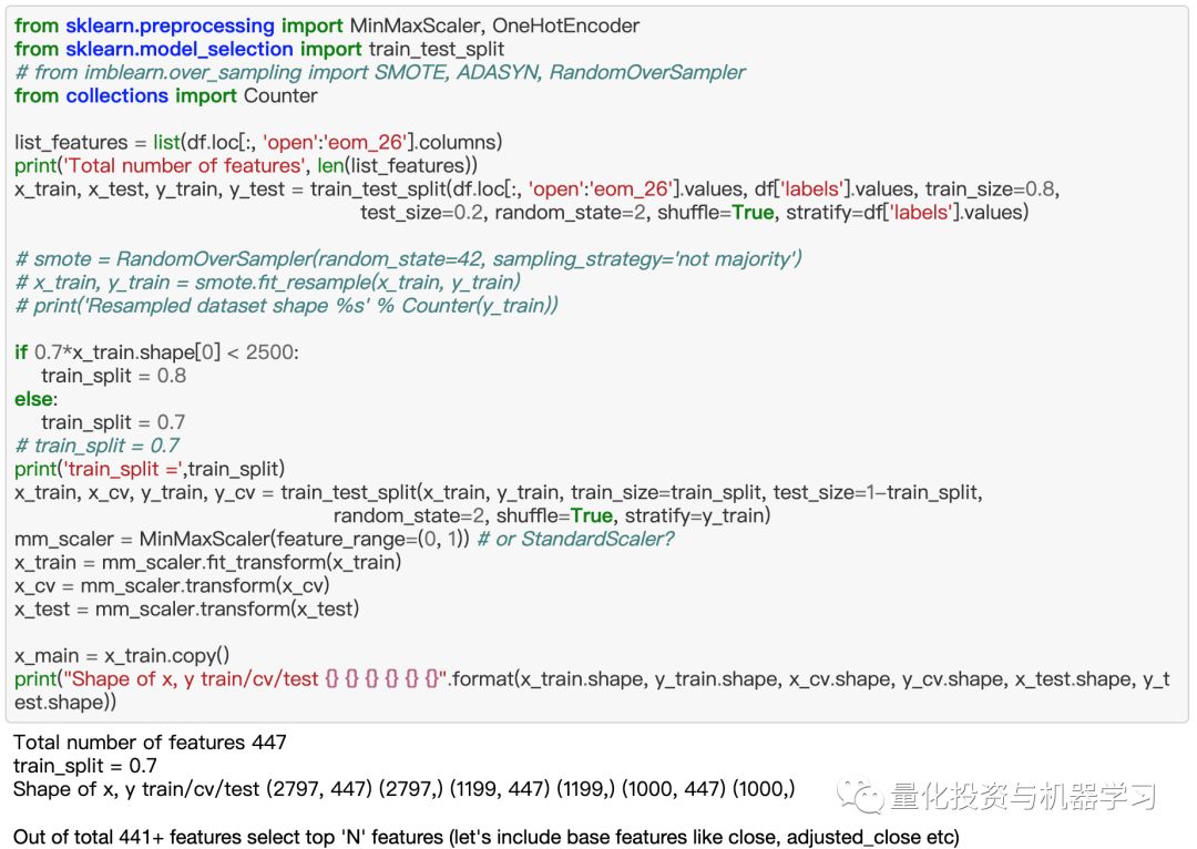
4. Normalization
We used Sklearn’s MinMaxScaler to normalize the data within the [0,1] range, although the paper used the [-1,1] range (the second deviation). It’s up to everyone’s preference.
5. Feature Selection
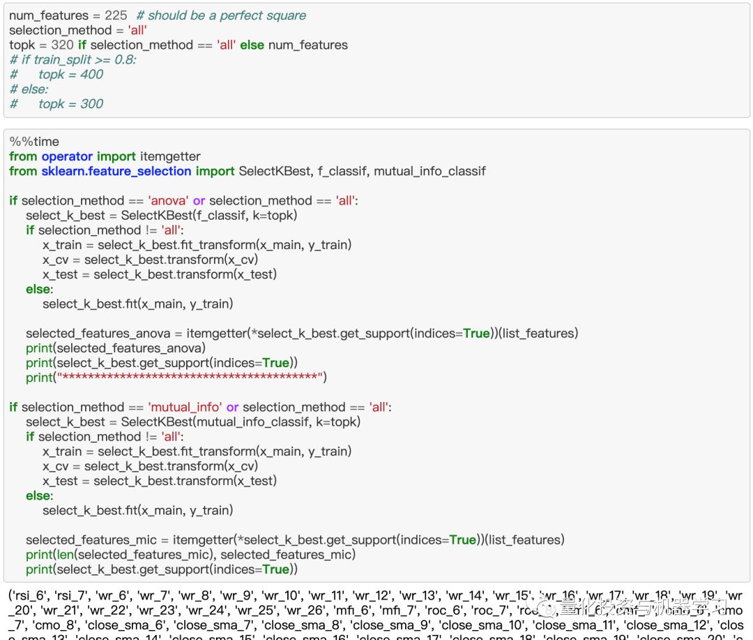
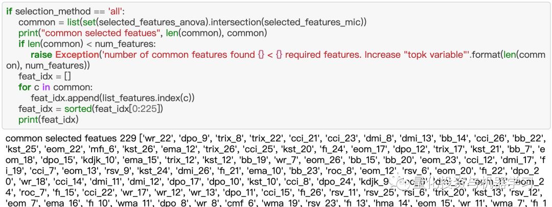
After calculating these indicators, we grouped them into images based on their types (momentum, oscillation, etc.) and trained many CNN architectures. We realized that the model was not learning enough, possibly due to insufficient quality of features. Therefore, we decided to adopt many other indicators instead of strictly following the calculation rules of different periods. We then applied feature selection techniques to choose 225 high-quality features. In fact, we used two feature selection methods: f_classif and mutual_info_classif, and selected the common features from their results. The original text did not mention feature selection (the third deviation).
···
···
Finally, we sorted the index list to find the intersection of f_classif and mutual_info_classif. This is to ensure that relevant features are very close in the image, and feature selection significantly improved the model’s performance.
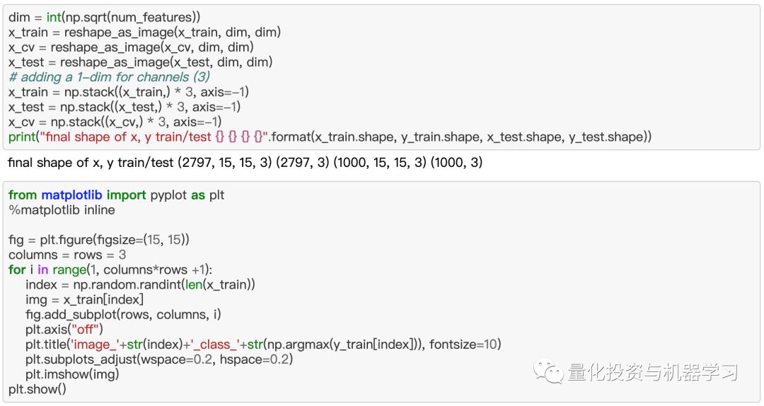
6. Mapping Data to Images
So far, we have a table containing 225 features. We need to convert it into images like this:
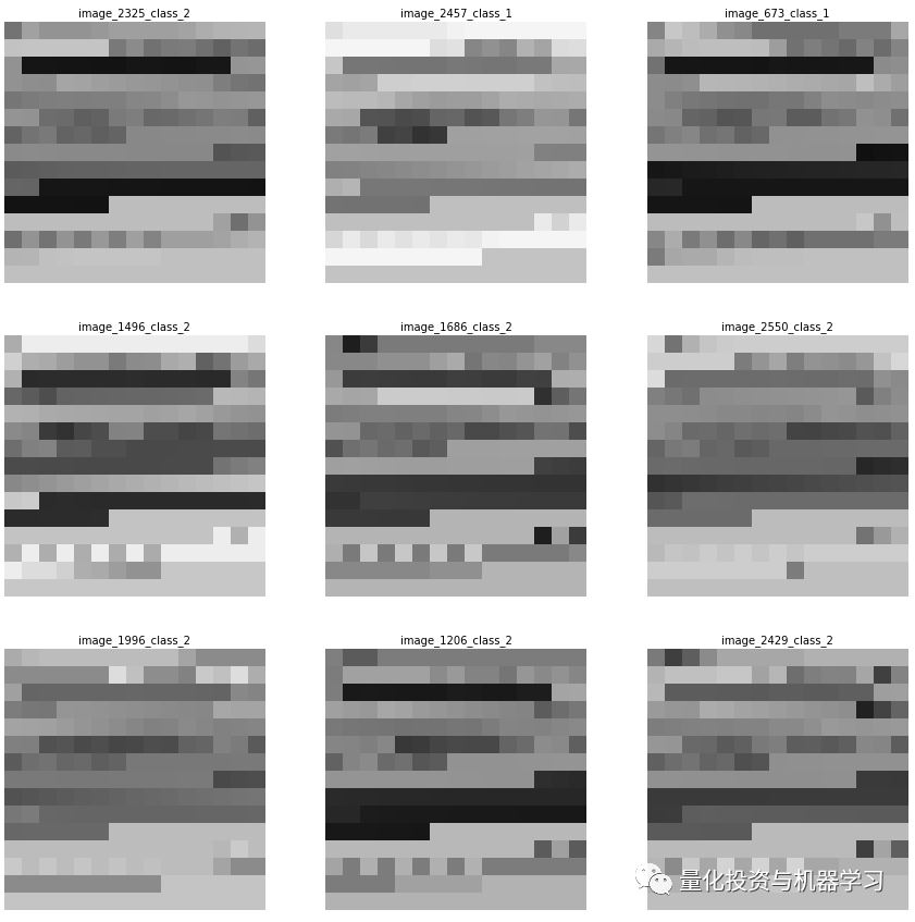
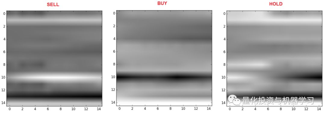
7. Addressing Imbalance
Another reason why this type of problem is difficult to solve is that the data is severely imbalanced. The number of “hold” instances is always far greater than buy/sell instances. In fact, the labeling algorithm proposed in this paper generates a considerable number of buy/sell instances. However, actual strategies tend to produce fewer instances.

It is very difficult for the model to learn anything meaningful. The paper only mentioned that “resampling” is one method to address this issue. We have tried oversampling (SMOTE, ADASYN), but none yielded satisfactory results. Ultimately, we opted for “sample weighting” (the fourth deviation). This is convenient for handling class imbalance. Here is how to calculate sample weights:
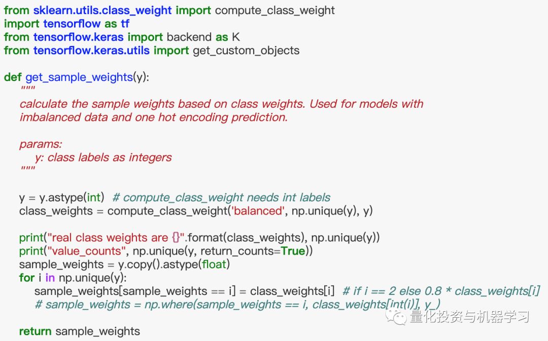
Then pass this sample weight array to the Keras fit function. You can also check the class_weights parameter.
8. Training
The model architecture mentioned in the paper is missing some details. For example, it does not mention the stride used. However, when we tried using stride=1 and padding=same, we realized that the model was too large, especially for training on 5 years of data. No matter how small the network we used, it was not good for sliding window training. Therefore, we decided to use cross-validation (the fifth deviation) for training on the full dataset. This part of the code includes rolling window training, all in the data_generator.py file.
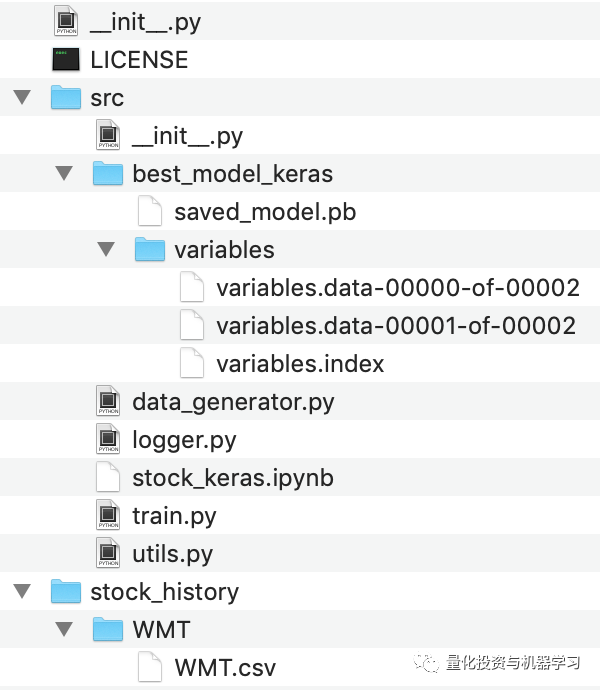
Get related code at the end of the article
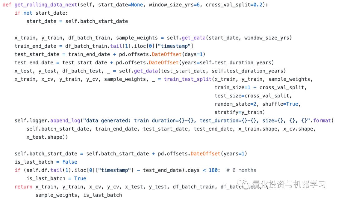
So far, the best CNN configuration we have found is:
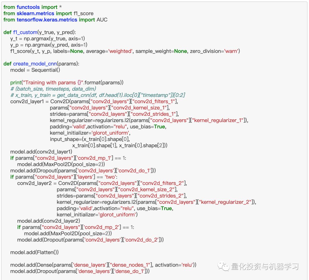
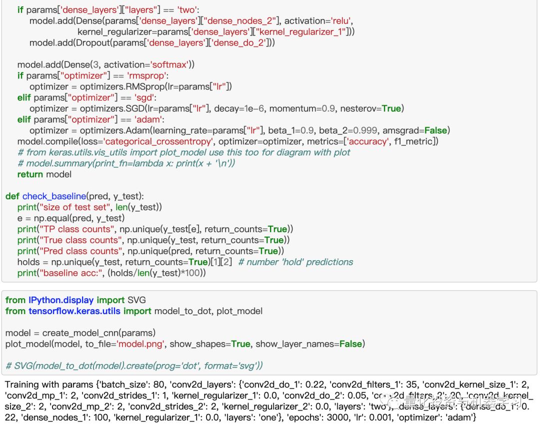

Keras model training is completed through early stopping and reduce_on_plateau callbacks, as shown below:
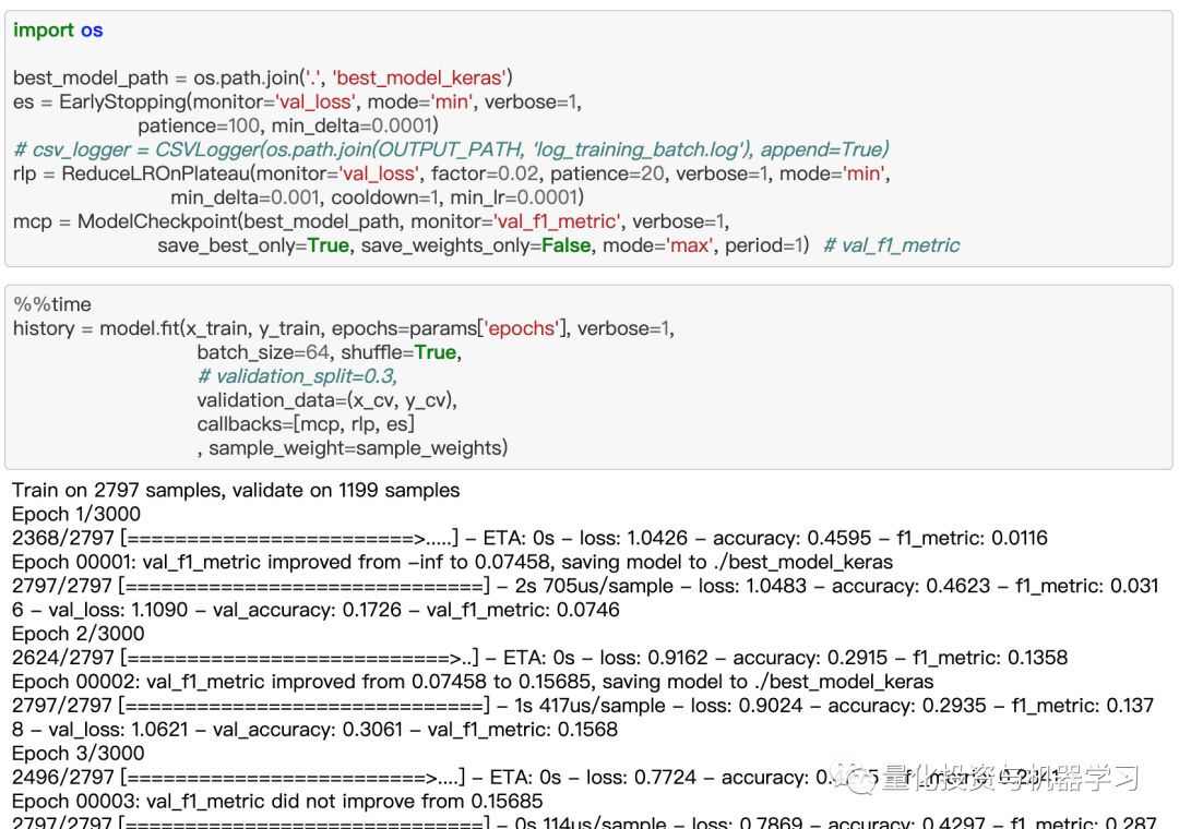
···
As you can see above, using the F1 score as a metric. For the evaluation of test data, we also used confusion matrix, Sklearn’s weighted F1 score, and Kappa.
Based on Walmart’s data, the above model produced the following results:
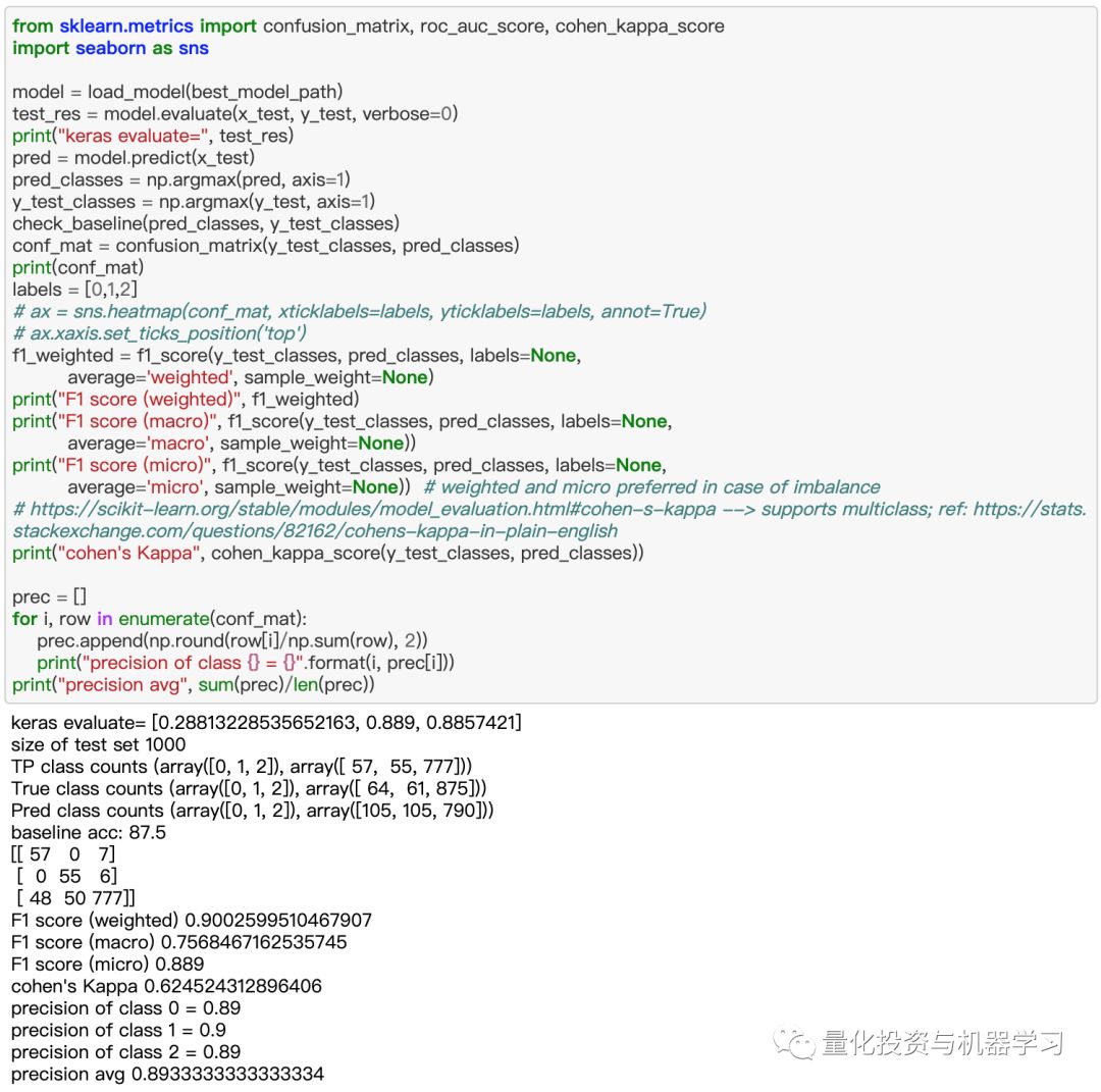
This result varies with each run, possibly due to Keras weight initialization. However, the accuracy values for each class remain in the range of [80,90], and the kappa value remains in the range of [58,65]. This is actually a well-known behavior, and specific discussions can be found here:
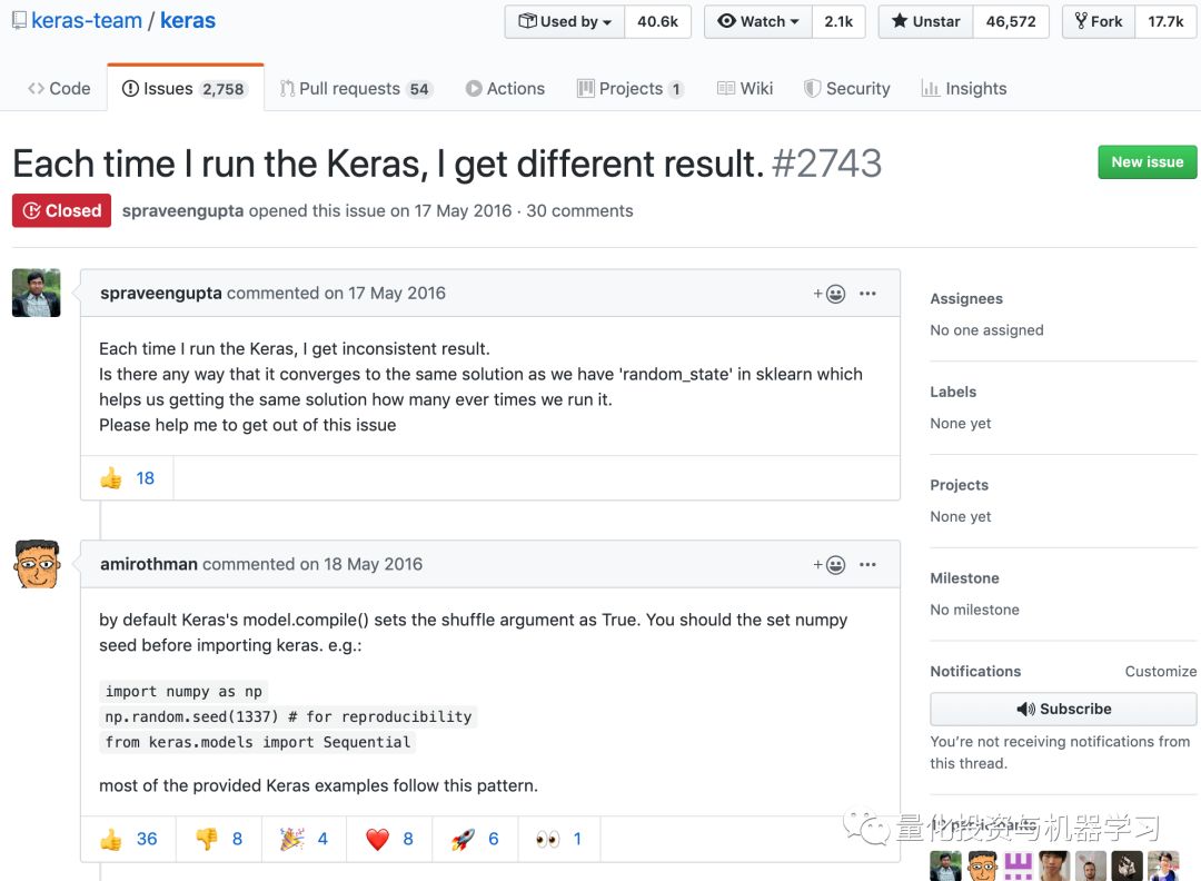
https://github.com/keras-team/keras/issues/2743
In short, you must set a random seed for Numpy and Tensorflow. We have set a random seed for numpy. So we are not sure if it solves the problem. But most of the time, for other CNN architectures we have tried, the accuracy of class 0 and class 1 (buy/sell) is lower than that of class 2 (class 0/1 is 80-85).
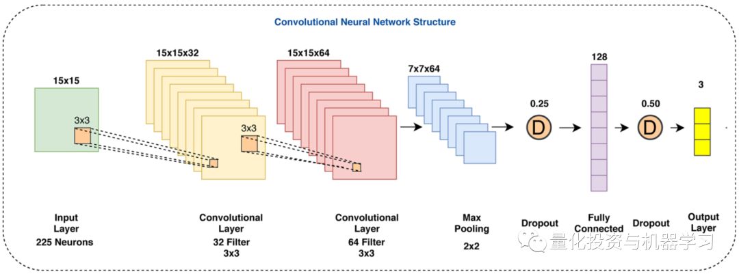
The model structure used by the authors has a similar structure (2 convolutional layers, dropout, dense layers [fully connected layers], etc.), but the results obtained are quite average (accuracy of 0.8 s for each class). Therefore, we had to adjust kernel sizes, dropout rates, and nodes to achieve better scores on the data. Here are the results published in the paper:

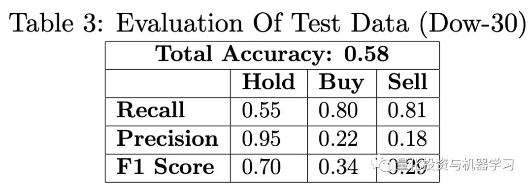
We think this result is quite good, as this model can recognize most buy/sell instances. Here are the authors’ views on this:
“However, a lot of false entry and exit points are also generated. This is mainly due to the fact that “Buy” and “Sell” points appear much less frequent than “Hold” points, it is not easy for the neural network to catch the “seldom” entry and exit points without jeopardizing the general distribution of the dominant “Hold” values. In other words, in order to be able to catch most of the “Buy” and “Sell” points (recall), the model has a trade-off by generating false alarms for non-existent entry and exit points (precision). Besides, Hold points are not as clear as “Buy” and “Sell” (hills and valleys). It is quite possible for the neural network to confuse some of the “Hold” points with “Buy” and “Sell” points, especially if they are close to the top of the hill or bottom of the valley on sliding windows.”
3
Further Improvements
Using the same CNN architecture on IBM data did not yield satisfactory buy/sell accuracy:
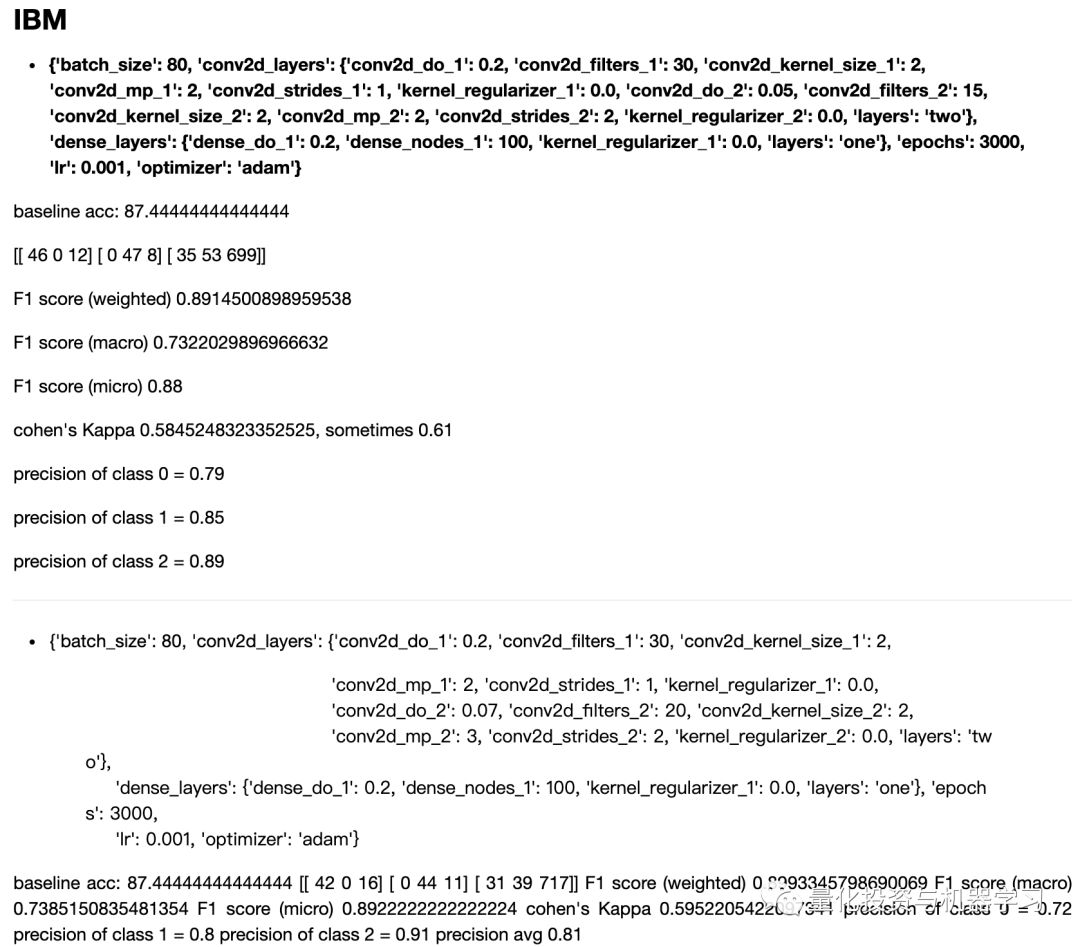
However, by adjusting hyperparameters, we can certainly improve it to a level similar to Walmart.
Although these results seem good enough, they do not guarantee profits in time trading, as they are limited by the data labeling strategy you choose. For example, when we backtested the above trading strategy (using original labels instead of model predictions), we did not make much profit.
Exploring other technical indicators may further improve the results.
Happy New Year to everyone! Recently, explore more without going out!
4
Get Code + Paper
Article No. 27 of 2020
The WeChat public account for quantitative investment and machine learning is a mainstream self-media in the industry focused on Quant, MFE, Fintech, AI, ML and other fields. The public account has more than 180,000+ followers from various circles, including public funds, private equity, brokerages, futures, banks, and insurance asset management. It publishes cutting-edge research results and the latest quantitative information daily.

