Four Fundamental Tasks of Computer Vision

Click on the above “Beginner’s Guide to Vision“, choose to add “Star” or “Top“

Important content delivered at the first time

Reprinted from: Author | Zhang Hao

Source | Zhihu(https://zhuanlan.zhihu.com/p/31727402)

Introduction:Deep learning has become one of the fastest-growing and most exciting fields of machine learning. Many significant papers have been published, and there are many high-quality open-source deep learning frameworks available. However, papers are often very concise and assume that readers have a considerable understanding of deep learning, which makes beginners often get stuck in understanding some concepts, reading papers with a sense of confusion, and finding it very difficult. On the other hand, even with easy-to-use deep learning frameworks, if one is not familiar with common concepts and basic ideas of deep learning, they will still be at a loss when facing real tasks and will not know how to design, diagnose, and debug networks.

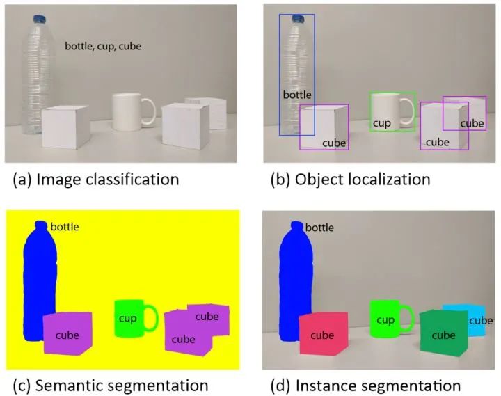
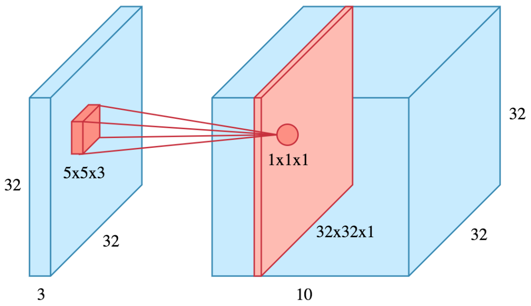
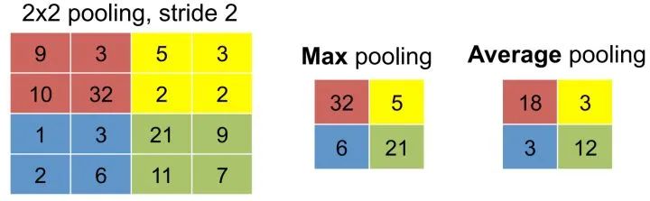
This series of articles aims to systematically sort out common concepts and basic ideas in various fields of deep learning, providing readers with an intuitive understanding of important concepts and ideas in deep learning, so as to achieve “knowing the reason behind it” and thus reduce the difficulty of understanding papers and practical applications later. This series of articles strives to describe in concise language, avoiding mathematical formulas and complicated details. This article is the second in this series, aiming to introduce the application of deep learning in the four fundamental tasks of computer vision, including classification (Fig. a), localization, detection (Fig. b), semantic segmentation (Fig. c), and instance segmentation (Fig. d). Subsequent articles will focus on the application of deep learning in other tasks in computer vision, as well as natural language processing and speech recognition.

(The author of this article is myself, and some content was first published in New Intelligence)

Introduction to Computer Vision

Computer vision aims to recognize and understand the content of images/videos. It originated from the “summer vision project” of the MIT AI Group in 1966. At that time, other branches of artificial intelligence had already achieved some preliminary results. Since humans can easily perform visual cognition, MIT professors hoped to solve computer vision problems through a summer project. Of course, computer vision was not solved in one summer, but after more than 50 years of development, it has become a very active research field. Today, over 70% of the data on the internet is images/videos, and the number of surveillance cameras worldwide has exceeded the population, generating more than 800 million hours of surveillance video data daily. Such a large volume of data urgently requires automated visual understanding and analysis technologies.

The difficulty of computer vision lies in the semantic gap. This phenomenon occurs not only in the field of computer vision; the Moravec paradox finds that high-level reasoning requires very little computational resources, while low-level perception of the external world requires a large amount of computational resources. It is relatively easy to get a computer to play chess like an adult, but it is quite difficult, if not impossible, to give a computer the perception and action capabilities of a one-year-old child.

The semantic gap means that humans can easily identify objects from images, while computers see images only as a set of integers between 0 and 255.

Other difficulties in computer vision tasks include variations in shooting angles, changes in the proportion of the target occupying the image, changes in lighting, background blending, target deformation, and occlusion.

Top conferences and journals in computer vision include CVPR, ICCV, and ECCV, and there are also many computer vision papers in ICLR. Due to the rapid development of the field of computer vision, it is essential for those in academia or industry to keep up with the latest research results by reading top conference and journal papers.

Convolutional Neural Networks (CNN)

The classic multilayer perceptron consists of a series of fully connected layers, while convolutional neural networks include convolutional layers and pooling layers in addition to fully connected layers.

(1) Convolutional Layer

Why use convolutional layers? The input images are usually very high-dimensional; for example, a 1,000×1,000 color image corresponds to three million-dimensional features. Therefore, continuing to use fully connected layers from multilayer perceptrons would lead to a huge number of parameters. A large number of parameters requires heavy computation and, more importantly, poses a higher risk of overfitting. Convolution is a locally connected, parameter-sharing version of a fully connected layer. These two features significantly reduce the number of parameters. The weights in the convolutional layer are often referred to as filters or convolutional kernels.

Local Connection In fully connected layers, each output is connected to all inputs through weights. In visual recognition, key image features, edges, corners, etc., only occupy a small part of the entire image, and the likelihood of two pixels that are far apart in the image affecting each other is very small. Therefore, in the convolutional layer, each output neuron is fully connected in the channel direction while only connected to a small part of input neurons in the spatial direction.

Shared Parameters If a set of weights can extract effective representations in a certain area of the image, they can also extract effective representations in other areas of the image. In other words, if a pattern appears in a certain area of the image, it can also appear in any other area of the image. Therefore, neurons at different spatial locations in the convolutional layer share weights to discover patterns in different spatial locations of the image. Shared parameters are an important idea in deep learning, allowing for a significant reduction in network parameters while still maintaining high network capacity. Convolutional layers share parameters in the spatial direction, while recurrent neural networks share parameters in the temporal direction.

Role of Convolutional Layers Through convolution, we can capture local information of the image. By stacking multiple convolutional layers, the features extracted by each layer gradually transition from low-level features such as edges, textures, and directions to high-level features such as text, wheels, and faces.

What is the relationship between convolution in convolutional layers and convolution in mathematics textbooks? There is basically no relationship. The convolution in convolutional layers is essentially the cross-correlation function of inputs and weights, rather than the convolution found in mathematics textbooks.

Four Quantities Describing Convolution The configuration of a convolutional layer is determined by the following four quantities: 1. Number of Filters. Using one filter to convolve the input will yield a two-dimensional feature map. We can use multiple filters to convolve the input to obtain multiple feature maps. 2. Receptive Field F, which is the size of the local connection in space for the filter. 3. Zero Padding P. As convolution proceeds, the image size will shrink, and information at the edges of the image will gradually be lost. Therefore, before convolution, we pad the image with some zeros on the top, bottom, left, and right, so that we can control the size of the output feature map. 4. Stride S. The filter computes an output neuron every S positions it moves in the input.

Relationship between Input and Output Sizes in Convolution Assuming the input height and width are H and W, and the output height and width are H‘ and W‘, then H‘=(H–F+2P)/S+1, W‘=(W–F+2P)/S+1. When S=1, by setting P=(F-1)/2, we can ensure that the input and output spatial sizes remain the same. For example, a 3*3 convolution requires padding of one pixel to keep the input and output spatial sizes unchanged.

What Size Filter Should Be Used It is advisable to use small filters, such as 3×3 convolutions. By stacking multiple layers of 3×3 convolutions, we can achieve the same receptive field as a large filter; for example, three layers of 3×3 convolutions are equivalent to a single layer of 7×7 convolution in terms of receptive field. However, using small filters has two benefits: 1. Fewer Parameters. Assuming the number of channels is D, the parameter count for three layers of 3×3 convolutions is 3×(D×D×3×3)=27D^2, while the parameter count for a single layer of 7×7 convolution is D×D×7×7=49D^2. 2. More Non-linearity. Since each convolutional layer is followed by a non-linear activation function, three layers of 3×3 convolutions pass through three non-linear activation functions, while a single layer of 7×7 convolution only passes through one.

1×1 Convolution is aimed at applying the same linear transformation to the D-dimensional vector at each spatial position. It is usually used to increase non-linearity or reduce dimensionality, which is an important way to reduce the computational burden and parameters of the network.

Fully Connected Layer Equivalent to Convolutional Layer Since both fully connected layers and convolutional layers perform dot products, these two operations can be equivalent. The equivalence of a fully connected layer to a convolutional layer requires setting the four quantities of the convolutional layer: the number of filters equals the number of output neurons in the original fully connected layer, the receptive field equals the spatial size of the input, no zero padding, and stride equals 1.

Why Equate Fully Connected Layers to Convolutional Layers Fully connected layers can only handle fixed-size inputs, while convolutional layers can handle inputs of any size. If the training image size is 224×224, and the test image size is 256×256, without the equivalence of fully connected layers to convolutional layers, we would need to crop multiple 224×224 regions from the test image to feed the network. After the equivalence, we only need to feed the 256×256 input through the network once to achieve the effect of multiple feeds of 224×224 regions.

Two Perspectives on Convolutional Results The convolutional result is a D×H×W three-dimensional tensor. It can be thought of as having D channels, each channel being a two-dimensional feature map that captures a specific feature from the input. It can also be thought of as having H×W spatial locations, each spatial location being a D-dimensional description vector that describes the semantic features of the local area of the image corresponding to the receptive field.

Distributed Representation of Convolutional Results The neurons of the convolutional results in different channels are not independent. There is a “many-to-many” mapping between the neurons of the convolutional results and semantic concepts, meaning that each semantic concept is represented by multiple channel neurons together, while each neuron also participates in multiple semantic concepts. Moreover, the neuron responses are sparse, meaning that most of the neurons output zero.

Implementation of Convolution Operations There are several basic ideas: 1. Fast Fourier Transform (FFT). By transforming to the frequency domain, convolution operations become ordinary matrix multiplications. In practice, this works well when the filter size is large, while for commonly used 1×1 and 3×3 convolutions, the acceleration is not significant. 2. im2col (image to column). im2col expands the local input area connected to each output neuron into a column vector and concatenates all resulting vectors into a matrix. This allows convolution operations to be implemented using matrix multiplication. The advantage of im2col is that it can utilize the efficient implementation of matrix multiplication, while the downside is that it consumes a large amount of storage because input elements appear multiple times in the generated matrix. Additionally, Strassen matrix multiplication and Winograd are often used. Existing computational libraries like MKL and cuDNN will choose appropriate algorithms based on filter size.

(2) Pooling Layer

The pooling layer down-samples based on local statistical information on the feature map, reducing the size of the feature map while retaining useful information. Unlike convolutional layers, pooling layers do not contain learnable parameters. Max pooling takes the maximum value in a local area as output, while average pooling calculates the mean of a local area as output. Max pooling is more commonly used in local area pooling, while global average pooling is a more commonly used global pooling method.

Role of Pooling Layers The pooling layer has the following three main functions: 1. Increase translation invariance of features. Pooling can enhance the network’s tolerance to minor displacements. 2. Reduce the size of the feature map. The pooling layer downsamples spatial local areas, reducing the number of parameters and computational load required in the next layer, and lowering the risk of overfitting. 3. Max pooling can introduce non-linearity. This is one of the reasons why max pooling is more commonly used. In recent years, some have used convolutional layers with a stride of 2 to replace pooling layers. In generative models, some studies have found that not using pooling layers makes the network easier to train.

Image Classification

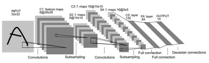
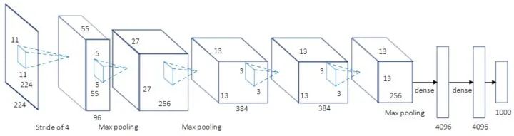
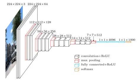
Given an input image, the image classification task aims to determine the category to which the image belongs.

(1) Common Datasets for Image Classification

Here are several commonly used classification datasets, arranged in increasing difficulty. rodrigob.github.io/are_ lists the performance rankings of various algorithms on each dataset.

MNIST 60k training images, 10k test images, 10 categories, image size 1×28×28, content is handwritten digits from 0-9.

CIFAR-10 50k training images, 10k test images, 10 categories, image size 3×32×32.

CIFAR-100 50k training images, 10k test images, 100 categories, image size 3×32×32.

ImageNet 1.2M training images, 50k validation images, 1k categories. From 2017 and prior, there was an annual ILSVRC competition based on the ImageNet dataset, which is equivalent to the Olympics in the field of computer vision.

(2) Classic Network Structures for Image Classification

Basic Architecture We use conv to represent convolutional layers, bn to represent batch normalization layers, and pool to represent pooling layers. The most common network structure order is conv -> bn -> relu -> pool, where convolutional layers are used to extract features, and pooling layers are used to reduce spatial size. As the network deepens, the spatial size of the image will decrease, while the number of channels will increase.

How to Design a Network for Your Task? When facing your actual task, if your goal is to solve that task rather than invent a new algorithm, do not attempt to design an entirely new network structure yourself, nor try to reproduce existing network structures from scratch. Look for publicly available implementations and pretrained models to fine-tune. Remove the last fully connected layer and corresponding softmax, add a fully connected layer and softmax corresponding to your task, and then freeze the preceding layers, only training the parts you added. If your training data is relatively abundant, you can fine-tune several layers, or even fine-tune all layers.

LeNet-5 60k parameters. The basic architecture of the network is: conv1 (6) -> pool1 -> conv2 (16) -> pool2 -> fc3 (120) -> fc4 (84) -> fc5 (10) -> softmax. The numbers in parentheses represent the number of channels, and the number 5 in the network name indicates that it has 5 layers of conv/fc layers. At that time, LeNet-5 was successfully used in ATMs to recognize handwritten digits in checks. LeNet is named after its author, LeCun.

AlexNet 60M parameters, the champion network of ILSVRC 2012. The basic architecture of the network is: conv1 (96) -> pool1 -> conv2 (256) -> pool2 -> conv3 (384) -> conv4 (384) -> conv5 (256) -> pool5 -> fc6 (4096) -> fc7 (4096) -> fc8 (1000) -> softmax. AlexNet has a similar network structure to LeNet-5, but is deeper and has more parameters. conv1 uses an 11×11 filter with a stride of 4, rapidly reducing the spatial size (227×227 -> 55×55). The key points of AlexNet are: (1). It uses the ReLU activation function, which provides better gradient properties and faster training. (2). It uses dropout. (3). It employs a large amount of data augmentation techniques. AlexNet is significant because it won the ILSVRC competition that year with a performance 10% higher than the runner-up, making people realize the advantages of convolutional neural networks. Additionally, AlexNet also made people aware that GPU acceleration could be used to speed up the training of convolutional neural networks. AlexNet is named after its author, Alex.

VGG-16/VGG-19 138M parameters, the runner-up network of ILSVRC 2014. The basic architecture of VGG-16 is: conv1^2 (64) -> pool1 -> conv2^2 (128) -> pool2 -> conv3^3 (256) -> pool3 -> conv4^3 (512) -> pool4 -> conv5^3 (512) -> pool5 -> fc6 (4096) -> fc7 (4096) -> fc8 (1000) -> softmax. The ^3 indicates that it is repeated 3 times. The key points of the VGG network are: (1). Simple Structure, consisting only of 3×3 convolutions and 2×2 pooling, and repeated stacking of the same module combinations. The convolutional layers do not change the spatial size, and every pooling layer halves the spatial size. (2). Large Number of Parameters, with most of the parameters concentrated in the fully connected layers. The number 16 in the network name indicates that it has 16 layers of conv/fc layers. (3). Proper network initialization and the use of batch normalization (BN) layers are crucial for training deep networks. In the original paper, it was impossible to directly train deep VGG networks, so shallow networks were first trained and used to initialize the deep networks. After BN appeared, along with other techniques, subsequent deep networks could be trained directly. VGG-19 has a structure similar to VGG-16, with slightly better performance than VGG-16, but VGG-19 consumes more resources, so VGG-16 is more commonly used in practice. Due to its very simple structure and suitability for transfer learning, VGG-16 is still widely used today. VGG-16 and VGG-19 are named after the research group the authors belong to (Visual Geometry Group).

GoogLeNet 5M parameters, the champion network of ILSVRC 2014. GoogLeNet attempts to answer what size of convolution or pooling layer should be chosen when designing a network. It proposes the Inception module, which simultaneously uses 1×1, 3×3, 5×5 convolutions and 3×3 pooling, retaining all results. The basic architecture is: conv1 (64) -> pool1 -> conv2^2 (64, 192) -> pool2 -> inc3 (256, 480) -> pool3 -> inc4^5 (512, 512, 512, 528, 832) -> pool4 -> inc5^2 (832, 1024) -> pool5 -> fc (1000). The key points of GoogLeNet are: (1). Multi-branch processing and concatenating results. (2). To reduce computational load, it uses 1×1 convolutions for dimensionality reduction. GoogLeNet uses global average pooling to replace fully connected layers, significantly reducing network parameters. GoogLeNet is named after the organization the authors belong to (Google), with the capital L paying homage to LeNet, and the Inception name coming from the