Exploring LSTM Networks in Stock Markets

LSTM Networks are a type of Recurrent Neural Network (RNN) first introduced by Sepp Hochreiter and Jurgen Schmidhuber in Neural Computation. After continuous improvement, the internal structure of LSTM has gradually become refined (Figure 1). It performs better than general RNNs when handling and predicting time series-related data. Currently, LSTM Networks are widely used in fields such as robotic control, text recognition and prediction, speech recognition, and protein homology detection. Based on the excellent performance of LSTM Networks in these areas, this article aims to explore whether LSTM can be applied to stock time series prediction.

Processing Stock Time Series

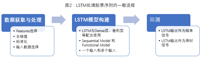
The LSTM processing flow for stock sequences used in this article is shown in Figure 2. The main library used to build the LSTM model is Keras.

Data Acquisition and Processing: For time series, we usually use the data of n moments as input to predict the output at moment (t+1), where the input is [X(t-n),X(t-n+1),…,X(t-1),X(t)]. For stocks, there will be several features at moment t. Therefore, to enrich the features for a more accurate model, this article uses a 2D vector of n(time series)×s(features per time series) as input. LSTM has high requirements for data normalization, so all input data in this article have undergone z-score normalization.

LSTM Model Construction: As a type of neural network structure in the recurrent layer, using only LSTM cannot construct a complete model; LSTM needs to be combined with other neural network layers (such as Dense layers, convolutional layers, etc.). Additionally, multiple LSTM layers can be constructed to increase the complexity of the model.

Backtesting: The backtesting conducted in this article is divided into two types: one is to directly use the LSTM output results as trading signals for backtesting on individual stocks, and the other is to use the LSTM prediction results as a timing signal, combined with other stock selection models (such as BigQuant’s StockRanker) for backtesting.

Previously, the public account published an article by Jakob Aungiers, who introduced the application of LSTM in Time Series Prediction in detail on his personal website (link [Click the title to view]：Time Series Prediction Using LSTM Neural Networks for Stock Markets), implemented on the BigQuant (https://bigquant.com) platform. The method used was to predict the next day’s closing price using the closing prices of the first 100 days of the CSI 300 index. From the results, LSTM’s prediction for the next 20 days is essentially a summary of the trend of closing price changes over the past 100 days, so the final prediction and backtesting results are not very ideal. Attempts to increase features (daily Open, High, Low, Close, Amount, Volume) also did not yield good results.

After analyzing the results and reading some research reports, the preliminary conclusion is that: first, the input time span is too long (the price trend of 100 days has little influence on the price change of the next day), while the predicted data time span is too short; second, the closing price (Close) is non-stationary data, and LSTM’s prediction performance on non-stationary data is not as good as on stationary data.

Considering the above two points, the inputs and outputs used in this article are based on using the past 30 days of data to predict the future five days’ returns.

Test Subject: CSI 300

Data Selection and Processing:

• The input time span is 30 days, with daily features being [‘close’,’open’,’high’,’low’,’amount’,’volume’] totaling 6, thus each input is a 30×6 2D vector.

• The output is the future five-day return future_return_5 (future_return_5>0.2, take 0.2; future_return_5<-0.2, take -0.2), for clearer training effects, output=future_return_5×10; features have all undergone standardization (each feature is standardized once within each sample).

• Training Data: Data for CSI 300 from January 1, 2005, to December 31, 2014; Testing Data: Data for CSI 300 from January 1, 2015, to May 1, 2017.

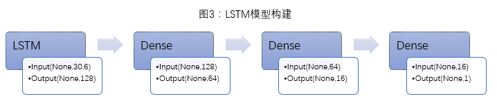
• Model Construction: Given the limited data (about 2500 training samples and about 500 prediction samples), the model construction is relatively simple. The model consists of one LSTM layer and three Dense layers (Figure 3).

• Backtesting: After obtaining the LSTM prediction results, if the LSTM predicted value is less than 0, it is recorded as -1, if greater than 0, it is recorded as 1.

Sample Code:

# Data processing: set each input (30 time series × 6 features) and data normalization
train_input = []
train_output = []
test_input = []
test_output = []
for i in range(conf.seq_len-1, len(traindata)):
    a = scale(scaledata[i+1-conf.seq_len:i+1])
    train_input.append(a)
    c = data['return'][i]
    train_output.append(c)
for j in range(len(traindata), len(data)):
    b = scale(scaledata[j+1-conf.seq_len:j+1])
    test_input.append(b)
    c = data['return'][j]
    test_output.append(c)

# LSTM accepts array type input
train_x = np.array(train_input)
train_y = np.array(train_output)
test_x = np.array(test_input) 
test_y = np.array(test_output)

# Custom activation function
import tensorflow as tf
def atan(x): 
    return tf.atan(x)

# Build neural network layers 1 LSTM layer + 3 Dense layers
# For 1 input situation
lstm_input = Input(shape=(30,6), name='lstm_input')
lstm_output = LSTM(128, activation=atan, dropout_W=0.2, dropout_U=0.1)(lstm_input)
Dense_output_1 = Dense(64, activation='linear')(lstm_output)
Dense_output_2 = Dense(16, activation='linear')(Dense_output_1)
predictions = Dense(1, activation=atan)(Dense_output_2)

model = Model(input=lstm_input, output=predictions)

model.compile(optimizer='adam', loss='mse', metrics=['mse'])

model.fit(train_x, train_y, batch_size=conf.batch, nb_epoch=10, verbose=2)

# Prediction
predictions = model.predict(test_x)

# Relationship between predicted values and true values
data1 = test_y
data2 = predictions
fig, ax = plt.subplots(figsize=(8, 6))
ax.plot(data2,data1, 'o', label="data")
ax.legend(loc='best')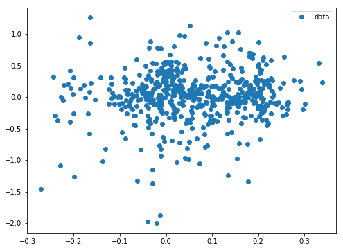

# If predicted value > 0, take as 1; if predicted value <= 0, take as -1. Prepare for backtesting
for i in range(len(predictions)):    
    if predictions[i]>0:
        predictions[i]=1
    elif predictions[i]<=0:
        predictions[i]=-1

# Combine predicted values with time as backtesting data
cc = np.reshape(predictions,len(predictions), 1)
databacktest = pd.DataFrame()
databacktest['date'] = datatime
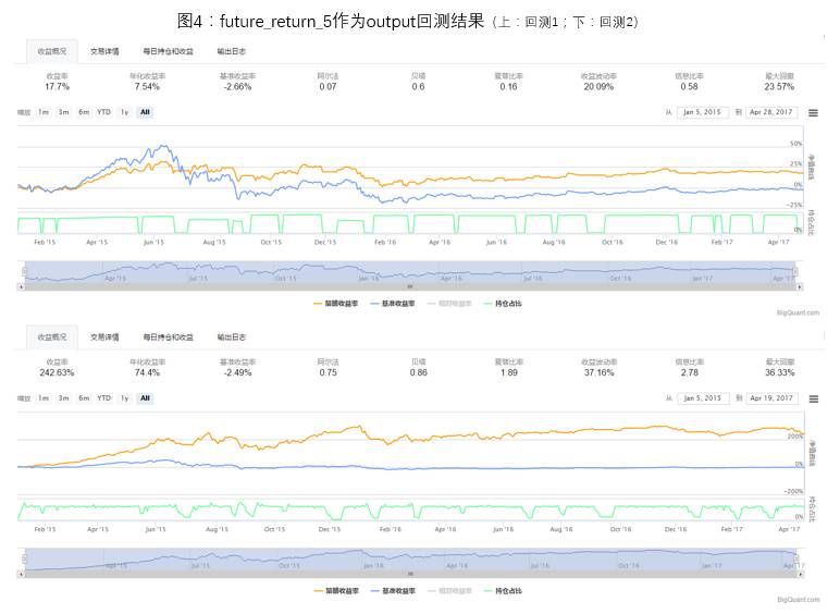
databacktest['direction']=np.round(cc)

Each model undergoes two backtests, the first backtest (hereafter referred to as backtest 1) directly uses the LSTM predicted values for trades on the CSI 300: if the LSTM predicted value is 1, buy and hold for 5 days (if already holding, update the holding days); if the LSTM predicted value is -1, if in a flat position, continue to hold flat, if already holding stocks, do not update the holding days;

The second backtest (hereafter referred to as backtest 2) uses LSTM as a timing indicator, combined with StockRanker for trading among 3000 stocks: if the LSTM predicted value is 1, allow StockRanker to buy stocks based on its ranking score; if the LSTM predicted value is -1, if in a flat position, continue to hold flat, if already holding stocks, prohibit StockRanker from buying stocks, and clear stocks within 5 days based on the buying time of existing stocks;

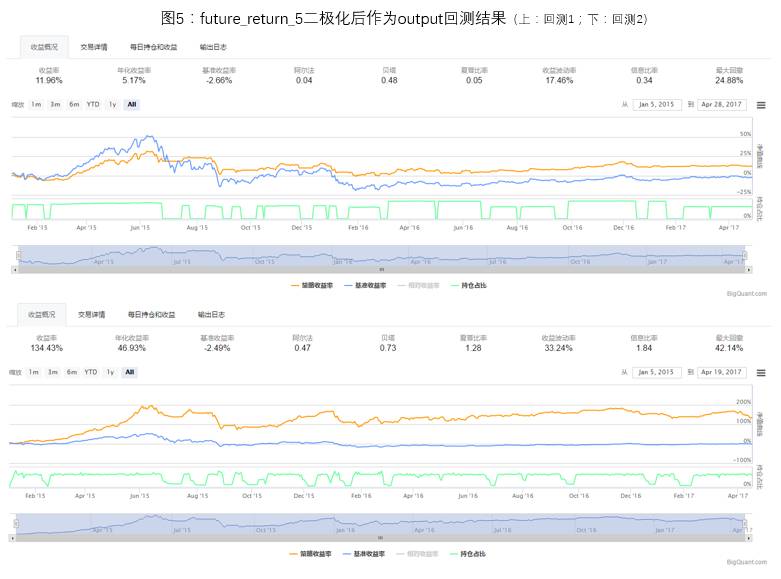
1) Comparison of Binary Processing of future_return_5

The processing of future_return_5 is divided into two situations, one is to directly use future_return_5 as output for model training, and the other is to binary process future_return_5 (future_return_5>0, take 1; future_return_5<=0, take -1), then use the binarized data as output for model training.

The backtesting situations for the two processing methods are shown in Figures 4 and 5. Due to the model’s weight initialization being different each time, the prediction and backtesting results will have some differences, but after multiple backtesting statistics, directly using future_return_5 as output for model training is a better choice. In the following discussions of this article, future_return_5 will be directly used as output for model training.

2) Exploring Regularization on Weights

Overfitting in Neural Networks: During the training of neural networks, “overfitting” is something to avoid. Overfitting means that the model performs well on the training data but poorly on predictions outside the training set. The reason is usually that the model “memorizes” the training data and its noise, leading to an overly complex model. The data volume for the CSI 300 used in this article is not very large, so preventing model overfitting is particularly important.

When training the LSTM model, there are two very important parameters at the parameter level that can control the model’s overfitting: Dropout parameters and applying regularization on weights. Dropout means randomly dropping some features during each input, thereby improving the model’s robustness. Its starting point is to change the network structure continuously so that the neural network learns not the training data itself but some regular patterns. Regularization is achieved by adding an L2 norm to the loss function calculation, causing some weight values to approach zero, preventing the model from forcibly adapting and fitting to each feature, thus improving robustness and having a factor selection effect; in the model training of 1), we added the Dropout parameter to avoid overfitting. Next, we will try additionally applying regularization on weights to test the model’s performance.

The backtesting results are shown in Figure 6. After adding regularization, the maximum drawdown in both backtest 1 and backtest 2 decreased, indicating that adding regularization indeed alleviated the model’s overfitting. Comparing the holding situation of backtest 1 before and after adding regularization, it can be seen that after adding regularization, the flat position duration is longer, and the number of trades decreases (19/17), which can be understood as: after adding regularization, the model becomes more conservative.

Issues with Regularization: Through experiments, for an LSTM model, the regularization parameter is very important, and tuning parameters requires a long time of trials. An inappropriate parameter choice can lead to the model’s predicted values being biased towards positive distribution (most predicted values greater than 0) or negative distribution, resulting in inaccurate prediction results, while better regularization parameters will make the model’s generalization very good (the model trained with the parameters used in Figure 6 has predicted values that belong to a mildly positive distribution). The discussions in this article will still be based on the LSTM model without weight regularization.

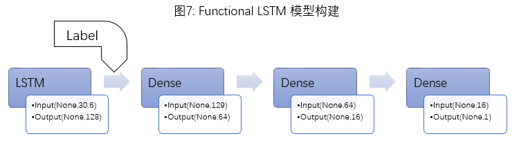
3) Exploring Dual Input Models

In addition to the traditional Sequential Model (one input, one output), this article also attempts to construct a Functional Model (supporting multiple inputs and outputs). The feature processing method mentioned earlier loses an important piece of information: the price level. The future_return_5 at the same input level could vary greatly when the index is at 3000 points versus 6000 points. Therefore, this article attempts to construct a “two inputs one output” Functional Model: standardized features are input into LSTM, and the output of the LSTM layer along with a label indicator (label=np.round(close/500)) is input into the subsequent Dense layer, with the final output still being future_return_5 (Figure 7).

Sample Code:

# LSTM and stock ranker combined backtesting
class conf:
    start_date = '2010-01-01'
    end_date='2017-05-01'
    # split_date: data before this date is for training, after for effect evaluation
    split_date = '2015-01-01'
    instruments = D.instruments(start_date, end_date)    
    label_expr = ['return * 100', 'where(label > {0}, {0}, where(label < -{0}, -{0}, label)) + {0}'.format(20)]    # Holding days, used to calculate return values in label_expr
    hold_days = 5

    # Features
    features = ['close_5/close_0',  # 5-day return
    'close_10/close_0',  # 10-day return
    'close_20/close_0',  # 20-day return
    'avg_amount_0/avg_amount_5',  # Today's/5-day average trading volume
    'avg_amount_5/avg_amount_20',  # 5-day/20-day average trading volume
    'rank_avg_amount_0/rank_avg_amount_5',  # Today's/5-day average trading volume ranking
    'rank_avg_amount_5/rank_avg_amount_10',  # 5-day/10-day average trading volume ranking
    'rank_return_0',  # Today's return
    'rank_return_5',  # 5-day return
    'rank_return_10',  # 10-day return
    'rank_return_0/rank_return_5',  # Today's/5-day return ranking
    'rank_return_5/rank_return_10',  # 5-day/10-day return ranking
    'pe_ttm_0',  # TTM price-earnings ratio
    ]
# Labeling data: scoring each row of data (sample), generally a higher score indicates better performance
m1 = M.fast_auto_labeler.v5(
    instruments=conf.instruments, start_date=conf.start_date, end_date=conf.end_date,
    label_expr=conf.label_expr, hold_days=conf.hold_days,
    benchmark='000300.SHA', sell_at='open', buy_at='open'
)

# Calculating feature data
m2 = M.general_feature_extractor.v5(
    instruments=conf.instruments, start_date=conf.start_date, end_date=conf.end_date,
    features=conf.features)

# Data preprocessing: handling missing data, data normalization, T.get_stock_ranker_default_transforms for StockRanker model data preprocessing
m3 = M.transform.v2(
    data=m2.data, transforms=T.get_stock_ranker_default_transforms(),
    drop_null=True, astype='int32', except_columns=['date', 'instrument'],
    clip_lower=0, clip_upper=200000000)

# Merging labeled data and feature data
m4 = M.join.v2(data1=m1.data, data2=m3.data, on=['date', 'instrument'], sort=True)

# Training dataset
m5_training = M.filter.v2(data=m4.data, expr='date < "%s"' % conf.split_date)

# Evaluation dataset
m5_evaluation = M.filter.v2(data=m4.data, expr='"%s" <= date' % conf.split_date)

# StockRanker machine learning training
m6 = M.stock_ranker_train.v2(training_ds=m5_training.data, features=conf.features)

# Predicting on evaluation set
m7 = M.stock_ranker_predict.v2(model_id=m6.model_id, data=m5_evaluation.data)

# Generating sell orders: selling starts after hold_days; for held stocks, the last ranked stock is eliminated based on StockRanker's prediction
if databacktest['direction'].values[databacktest.date==current_dt]==-1: # LSTM timing sell
    instruments = list(reversed(list(ranker_prediction.instrument[ranker_prediction.instrument.apply(lambda x: x in equities and not context.has_unfinished_sell_order(equities[x]))])))        
     for instrument in instruments:            
         if context.trading_calendar.session_distance(pd.Timestamp(context.date[instrument]), pd.Timestamp(current_dt))>=5:
                context.order_target(context.symbol(instrument), 0)if not is_staging and cash_for_sell > 0:
    instruments = list(reversed(list(ranker_prediction.instrument[ranker_prediction.instrument.apply(lambda x: x in equities and not context.has_unfinished_sell_order(equities[x]))])))        
    # print('rank order for sell %s' % instruments)    for instrument in instruments:
        context.order_target(context.symbol(instrument), 0)
        cash_for_sell -= positions[instrument]            
        if cash_for_sell <= 0:                
            break
            
# Generating buy orders: buying stocks based on StockRanker's prediction ranking, only for the first stock_count stocks
if databacktest['direction'].values[databacktest.date==current_dt]==1: # LSTM timing buy
    buy_dt = data.current_dt.strftime('%Y-%m-%d')
    context.date=buy_dt
    buy_cash_weights = context.stock_weights
    buy_instruments = list(ranker_prediction.instrument[:len(buy_cash_weights)])
    max_cash_per_instrument = context.portfolio.portfolio_value * context.max_cash_per_instrument        
    for i, instrument in enumerate(buy_instruments):
        cash = cash_for_buy * buy_cash_weights[i]            
        if cash > max_cash_per_instrument - positions.get(instrument, 0): # Ensure stock holding amount does not exceed the maximum cash occupied by each stock
            cash = max_cash_per_instrument - positions.get(instrument, 0)            
        if cash > 0:
            context.order_value(context.symbol(instrument), cash)
            buy_dates[instrument] = current_dt

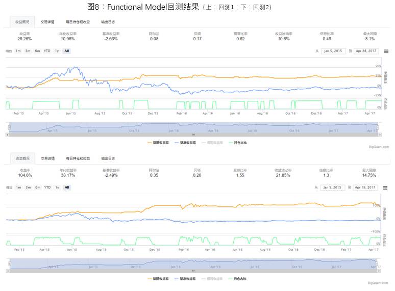
context.date = buy_dates

Backtesting results are shown in Figure 8. From the backtesting results, it can be seen that the return rate of the LSTM model with the indicator label is relatively lower, but the drawdown is smaller. The time periods when the LSTM predicted value is less than 0 cover most of the significant declines in the CSI 300, although it also mistakenly classifies some oscillating or rising trends as declining trends. Perhaps this is unavoidable; as the saying goes, high risk leads to high returns, and low risk means that returns won’t be very high. High returns and low risk are often mutually exclusive.

Conclusion: This article explores the application of LSTM to predict the future five-day returns of the CSI 300, initially indicating that LSTM Networks can be used in the stock market. Since LSTM is more suitable for handling individual stocks/indices, using LSTM as a timing model in combination with other stock selection models performs better. Using the LSTM model to predict CSI 300 data and taking the results as timing signals can significantly improve the drawdown of the stock ranker stock selection model during backtesting.

Outlook: Due to the limited data volume for individual stocks, the scalability and complexity of the LSTM model are greatly constrained, and the selection of features is also limited (if the input features are too many while the data is limited, some features may not be able to perform their due functions, which is also prone to overfitting). In the future, we hope to test the performance of LSTM on hourly or minute data for individual stocks/indices. Additionally, exploring whether the LSTM model can process the data of all stocks belonging to an industry together is also a potential direction.

Note: Due to the different weight update situations during each training of the LSTM model and the randomness of Dropout, the training results of the LSTM model will vary each time.

Tip: Since LSTM involves numerous parameters, we cannot guarantee the stability of the LSTM model at present. The backtesting results attached to this article are all selected from relatively ideal situations after multiple model training, aiming to demonstrate that LSTM can be applied to the stock market and that it is possible to use it as a timing model. The discussions and codes provided in this article are for exploration and discussion only. To form a more practical LSTM model in the stock market, significant effort is still needed in feature selection, model construction, parameter selection, and tuning.