Essential Guide to LSTM: From Basics to Functionality Explained

Selected from echen

Translated by Machine Heart

Contributors: Machine Heart Editorial Team

Long Short-Term Memory (LSTM) is a crucial neural network technology that has been widely applied in many fields, including speech recognition and natural language processing. In this article, Edwin Chen provides a systematic introduction to LSTM. Machine Heart has translated this article.

The first time I learned about LSTM, it caught my eye. It turns out that LSTM is a relatively simple extension of neural networks, and behind the astonishing achievements of deep learning in recent years, they all have its shadow. So I will present them as intuitively as possible—so that you can figure it out for yourself.

First, let’s take a look at a diagram:

LSTM is beautiful, isn’t it? Let’s get started!

(Tip: If you are already familiar with neural networks and LSTM, feel free to skip to the middle section; the first half of this article is an introductory overview.)

Neural Networks

Imagine we have a sequence of images from a movie, and we want to label each image with an action (for example, is there a fight? Are the characters talking? Is someone eating in the picture…)

How do we do that?

One way is to ignore the sequential nature of the images and construct an image classifier that considers each image separately. For instance, when provided with enough images and labels:

• Our algorithm first detects lower-level patterns, such as shapes and edges.

• With more data, it may learn to combine these patterns into more complex patterns, such as faces (two round things with a triangle below and an oval below that) or cats.

• Even with more data, it may learn to map these high-level patterns to the actions themselves (a scene with a mouth, steak, and fork may relate to eating).

So, that’s a deep neural network: it takes an image as input and returns an action as output, just like we can learn to detect patterns in dog behavior without knowing anything about dogs (after seeing enough corgis, we notice things like fluffy butts and stubby legs), a deep neural network can learn to represent images through the representations of hidden layers.

Mathematical Description

I assume the reader is already familiar with basic neural networks, so let’s quickly review.

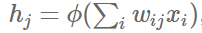
• A neural network with only a single hidden layer takes a vector x as input; we can think of it as a set of neurons.

• Each input neuron is connected to the hidden layer through a set of learned weights.

• The output of the j-th hidden neuron is as follows: (where ϕ is an activation function)

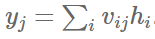
• The hidden layer is fully connected to the output layer, and the output yj of the j-th output neuron is as follows: if we need to output probabilities, we can transform the output using the softmax function.

Written in matrix form as follows:

Where

• x is the input vector

• W is the weight matrix connecting the input to the hidden layer

• V is the weight matrix connecting the hidden layer to the output

• Common activation functions ϕ are the sigmoid function σ(x), which compresses numbers in the range (0,1); the hyperbolic tangent function (tanh(x)), which compresses numbers in the range (-1,1); and the rectified linear unit function, ReLU(x)=max(0,x).

Next, let’s describe a neural network with a diagram:

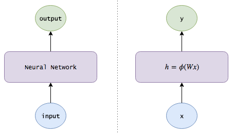
(Note: To simplify the notation, I assume x and h each contain an additional bias neuron with a fixed value of 1.)

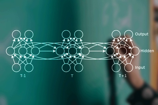
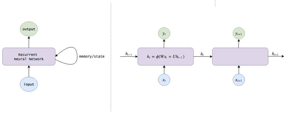
Using Recurrent Neural Networks (RNN) to Remember Information

However, ignoring the sequential information of movie images is just the simplest machine learning. If we see a scene of a beach, we should emphasize the activities on the beach in later frames: an image of someone in the water should be more likely labeled as swimming rather than bathing; an image of someone lying with their eyes closed should be more likely labeled as sunbathing. If we remember that Bob just arrived at a supermarket, then even without any specific supermarket features, a photo of Bob holding a piece of bacon should be more likely classified as shopping rather than cooking.

So what we want is for our model to track the state of the world:

1. After viewing each image, the model outputs a label and updates its knowledge about this world. For example, the model may learn to automatically discover and track positions (is the current scene indoors or at the beach?), the time of day (if the scene contains the moon, then the model should remember it is night), and the progress of the movie (is this the first image or the 100th frame?). Crucially, just as the neural network can automatically discover hidden edges, shapes, and faces in images without being fed information, our model should also rely on itself to discover some useful information.

2. When given a new image, the model should combine the knowledge it has already collected to perform better.

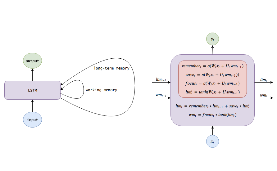
This is a Recurrent Neural Network (RNN). In addition to simply inputting an image and returning an action label, RNN also maintains internal knowledge about the world (the weights assigned to different pieces of information) to assist in executing its classification.

Mathematical Description

So, let’s incorporate the concept of internal knowledge into our equations, and we can think of internal memory as the memory of information fragments that the network maintains over time.

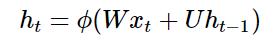
But this is easy: we know that the hidden layers of neural networks have already encoded useful information from the input, so why not use these hidden layers as memory? This gives us our RNN equations:

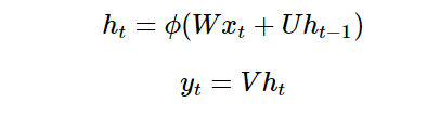
Note that the hidden state ht computed at time t (ht is our internal knowledge here) will be fed back into the next time step. (Additionally, I will use terms such as hidden state, knowledge, memory, and belief interchangeably to describe ht)

Implementing Longer Memory with LSTM

Let’s think about how the model updates its knowledge about the world. So far, we haven’t imposed any constraints on this update, so its knowledge may become very chaotic: in one frame, it thinks a person is in the USA, and in the next frame, it sees someone eating sushi, so it thinks the person is in Japan, and in the subsequent frame, it sees a polar bear, so it thinks they are on Wrangel Island. Or perhaps it has a lot of information indicating that Alice is an investment analyst, but after seeing her culinary skills, it concludes she is a professional killer.

This chaos means information is rapidly shifting and disappearing, making it difficult for the model to maintain long-term memory. So what we want is for the network to learn how to evolve its knowledge about the world in a more gentle way, thereby updating its beliefs (the scene without Bob should not change the information about Bob, while the scene containing Alice should focus on collecting some details about her).

Here are four ways we can do this:

1. Add a forgetting mechanism: if a scene ends, the model should forget the positions, times of day, and reset any information related to the scene; however, if a person in the scene dies, the model should always remember that the deceased person is no longer alive. Therefore, we want the model to learn a discriminative forgetting/memory mechanism: when new input arrives, it needs to know which beliefs to remember and which to discard.

2. Add a saving mechanism: when the model sees a new image, it needs to learn whether the information about this image is worth using and saving. Perhaps your mom gave you an article about Kylie Jenner, but who cares?

3. So when new input arrives, the model first needs to forget any long-term memory information it considers no longer necessary. Then it learns which parts of the new input are worth utilizing and saves them in its long-term memory.

4. Focus long-term memory on working memory: finally, the model needs to learn which parts of long-term memory are immediately useful. For example, Bob’s age may be a piece of information that needs to be retained long-term (children are likely playing, while adults are likely working), but if he is not in the current scene, then this information is likely not particularly relevant. So the model learns to focus on which part, rather than always utilizing the complete long-term memory.

This is a Long Short-Term Memory network (LSTM). LSTM passes memory in a very precise way—using a specific learning mechanism: which parts of information need to be remembered, which parts need to be updated, and which parts need to be attended to. In contrast, recurrent neural networks rewrite memory in an uncontrolled manner at each time step. This helps track information over longer periods.

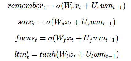
Mathematical Description

Let’s provide a mathematical description of LSTM.

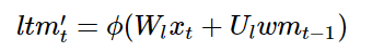
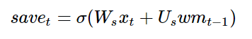
At time t, we receive new input xt. We also have our long-term memory and working memory carried over from previous time steps, ltm(t−1) and wm(t−1) (both are n-dimensional vectors), which are what we want to update.

We will start with our long-term memory. First, we need to know which long-term memories need to be kept and which need to be discarded, so we want to use the new input and our working memory to learn a memory gate composed of n numbers between 0 and 1, each number determining how much of a long-term memory element is kept. (1 means fully kept, 0 means fully discarded.)

Naturally, we can use a small neural network to learn this memory gate:

(Note the similarity to our previous neural network equations; this is just a shallow neural network. Additionally, we used the sigmoid activation function because the numbers we need are between 0 and 1.)

Next, we need to calculate the information we can learn from xt, which is our candidates for long-term memory:

Where ϕ is an activation function, typically chosen as the hyperbolic tangent function.

However, before we add this candidate to our memory, we want to learn which parts are actually worth using and saving:

(Think about what happens when you read something on a webpage. When a news article might contain information about Hillary, if the source is Breitbart, you should ignore it.)

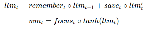
Now let’s combine all these steps together. After forgetting what we think we won’t use again and saving useful new information, we have updated long-term memory:

Next, to update our working memory: we want to learn how to focus our long-term memory on the information that will be immediately useful. (In other words, we want to learn how to move which information from external storage to the working memory on our notebook.) So we will learn a focus/attention vector:

Then our working memory becomes:

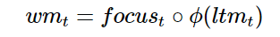
In other words, we focus entirely on elements with a focus of 1, ignoring those with a focus of 0.

Then our work on long-term memory is complete! And hopefully, this can be called your long-term memory.

Summary: A standard RNN updates hidden states/memory with a single equation:

Whereas LSTM uses several equations:

Each memory/attention sub-mechanism is just a mini version of LSTM:

(Note: The terms and variable names I use here differ from those in the usual literature. Here are some standard names that I will interchangeably use later:

• Long-term memory ltm(t), usually referred to as cell state, abbreviated c(t).

• Working memory wm(t), usually referred to as hidden state, abbreviated h(t). This is similar to the hidden state in standard RNNs.

• Memory vector remember(t), usually referred to as forget gate (although in the forget gate, 1 still means fully retaining memory and 0 means fully forgetting), abbreviated f(t).

• Saving vector save(t), usually referred to as input gate (as it determines how much of the input is allowed into the cell state), abbreviated i(t).

• Attention vector focus(t), usually referred to as output gate, abbreviated o(t).

Snorlax

At the time of writing this blog post, I could have caught a hundred Pidgeys; please see the comic below.

Neural Networks

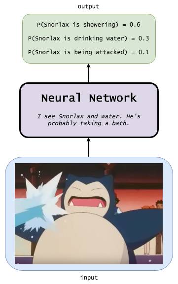
The neural network determines with a probability of 0.6 that the Snorlax in the input image is showering, with a probability of 0.3 that it is drinking water, and with a probability of 0.1 that it is being attacked.

Recurrent Neural Networks

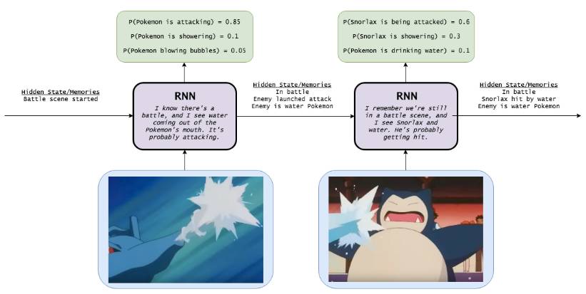
When a recurrent neural network is used to do this, it has memory of the previous image. The final result is a probability of 0.6 that Snorlax is being attacked, 0.3 that it is showering, and 0.1 that it is drinking water. The result is significantly better than the neural network in the previous image.

LSTM

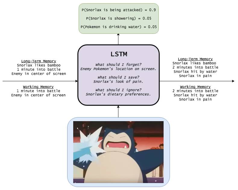
With long-term memory, LSTM increases the probability of accurately describing the scene in the cartoon image to 0.9, given that it remembers various relevant information.

Learn to Program

Let’s look at some examples of what an LSTM can do. Following the brilliant blog post by Andrej Karpathy (http://karpathy.github.io/2015/05/21/rnn-effectiveness/), I will use a character-level LSTM model that takes sequences of characters as input and is trained to predict the next character in the sequence.

While this seems a bit of a joke, character-level models are indeed very useful, even more so than word-level models. For example:

• Imagine an auto-programmer smart enough to allow you to program on your phone. In theory, an LSTM model could track the return type of the function you are currently in, allowing it to better suggest you return that variable; it could also know whether you have created a bug just by the returned error type without going through compilation.

• Natural language processing applications like machine translation often struggle with rare entries. How do you translate a word you’ve never seen before, or how do you convert an adjective into a verb? Even if you know the meaning of a tweet, how do you generate a new label to describe it? Character-level models can dream up new items, so this is another area with interesting applications.

So here we go, I launched an EC2 p2.xlarge spot instance and trained a 3-layer LSTM model on the Apache Commons Lang codebase (link: https://github.com/apache/commons-lang). Below is the program generated a few hours later:

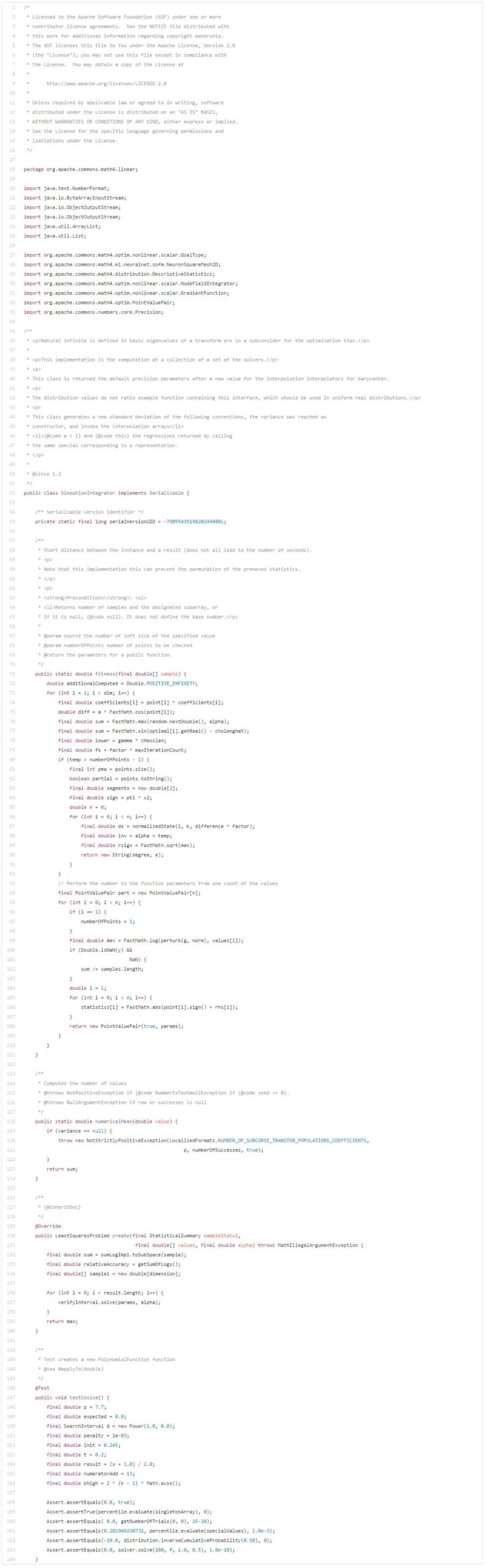
Although this code is not perfect, it is better than what many data scientists I know would produce. We can see that LSTM has learned many interesting (and correct!) programming behaviors.

• It understands how to construct classes: the top has license-related information, followed by package and import, then comments and class definitions, and finally variables and functions. Similarly, it knows how to create functions: comments follow the correct order (description, then @param, then @return, etc.), decorators are placed correctly, and non-empty functions can end with appropriate return statements. The key is that this behavior spans large blocks of code—you can see how large the code blocks are in the image!

• It can also track subroutines and nesting levels: indentation is always correct, and if statements and for loops are always handled well.

• It even knows how to construct tests.

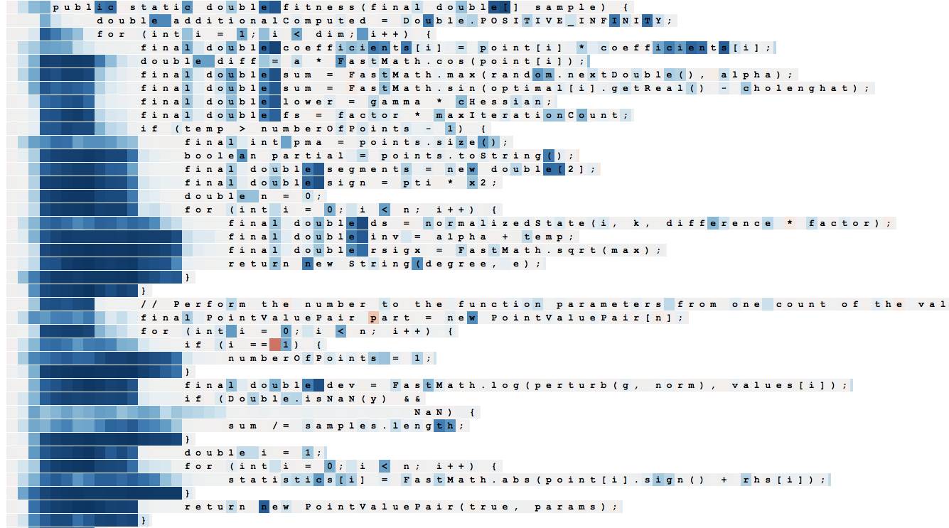
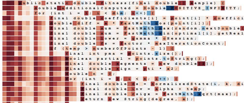
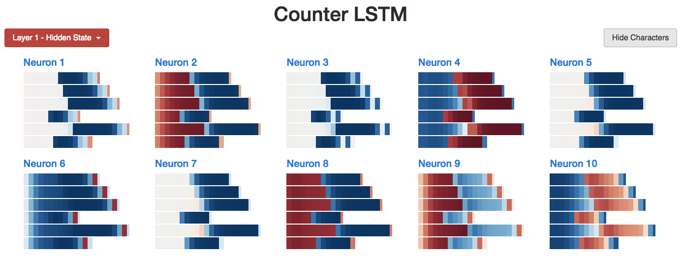
So how does the model achieve this? Let’s take a look at a few hidden states.

Below is a neuron that seems to be tracking the outer indentation of the code (when reading characters as input, meaning that when trying to generate the next character, each character is colored according to the neuron state; red units are negative, blue units are positive):

Below is a neuron that counts the number of spaces:

For fun, below is the output of another different 3-layer LSTM model trained on the TensorFlow codebase:

There are many interesting examples online, so if you want to learn more, please check: http://karpathy.github.io/2015/05/21/rnn-effectiveness/

Exploring the Internals of LSTM

Let’s dig a little deeper. We will look at the previous hidden state examples, but I also want to play with LSTM cell states and other memory mechanisms. We expect them to either spark or produce surprising visuals?

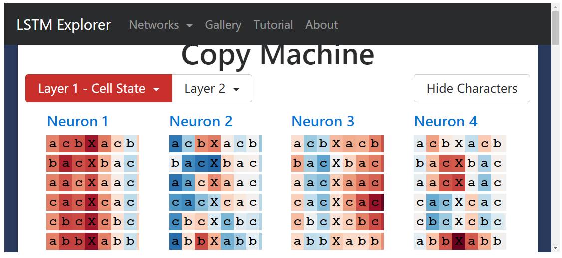
Counting

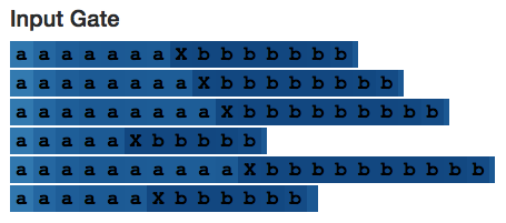
To study, let’s start by teaching an LSTM to count. (You should remember how the LSTM models in Java and Python learned to generate appropriate indentation!) So I generated sequences of the following form:

aaaaaXbbbbb

(N letters “a”, followed by a letter separator X, followed by N letters “b”, where 1 <= N <= 10), and then trained a single-layer LSTM with 10 hidden neurons.

Not surprisingly, the LSTM model learned perfectly during training—even able to generalize the generation to a few steps beyond. (Even at the start when we tried to make it remember 19, it failed.)

aaaaaaaaaaaaaaaXbbbbbbbbbbbbbbb
aaaaaaaaaaaaaaaaXbbbbbbbbbbbbbbbb
aaaaaaaaaaaaaaaaaXbbbbbbbbbbbbbbbbb
aaaaaaaaaaaaaaaaaaXbbbbbbbbbbbbbbbbbb
aaaaaaaaaaaaaaaaaaaaXbbbbbbbbbbbbbbbbbb # Here it begins to fail: the model is given 19 "a"'s, but outputs only 18 "b"'s.

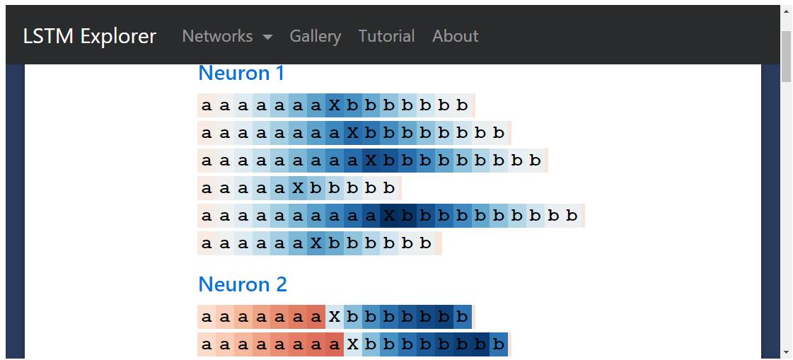
We expect to find a hidden state neuron that counts each a as we observe the model internally. Just as we did:

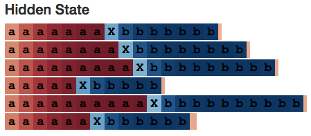
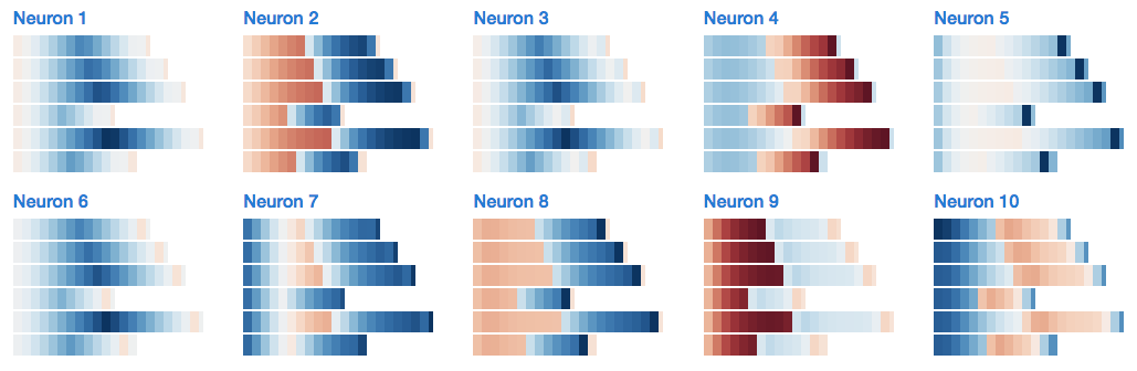
I developed a small web app that allows you to play with LSTM, and neuron #2 seems to be able to keep track of the number of a’s seen as well as the number of b’s seen. (Remember, the unit’s color is based on the activation level, from deep red [-1] to deep blue [+1].)

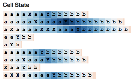
So what about the cell state? Its behavior looks something like this:

Interestingly, working memory is like a “sharpened version” of long-term memory. But is this generally the case?

It indeed is. (I expected as much because long-term memory is compressed by the hyperbolic tangent activation function, and the output gate restricts the content that passes through it.) For example, the following image shows the states of all 10 cells at a certain moment. We see many cells with very faint colors, which represents their values being close to 0.

In contrast, the 10 working memory neurons look much more focused. Neurons 1, 3, 5, and 7 are even all 0 in the first half of the sequence.

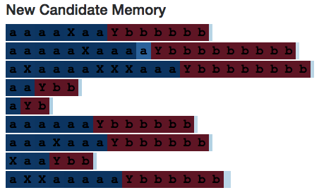
Let’s return to neuron #2. Here are some candidate memory and input gates. They remain relatively unchanged in the first or second half of each sequence—it’s as if the neuron is computing a+=1 or a-=1 at each step.

Finally, here is an overall view of neuron 2:

If you want to explore different counting neurons yourself, you can play around with this visualization web app.

(Note: This is far from the only way an LSTM model can learn to count; I am only describing one here. However, I think observing network behavior is interesting, and it helps build better models; after all, many ideas in neural networks come from the human brain. If we see unexpected behavior, we might be able to design more effective learning mechanisms.)

Counting from Counting

Let’s look at a slightly more complex counter. This time, I generated sequences of the following form:

aaXaXaaYbbbbb

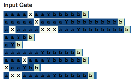
(N a’s with X randomly inserted in between, followed by a separator Y, followed by N b’s.) The LSTM still needs to count the number of a’s, but this time it needs to ignore the number of X’s.

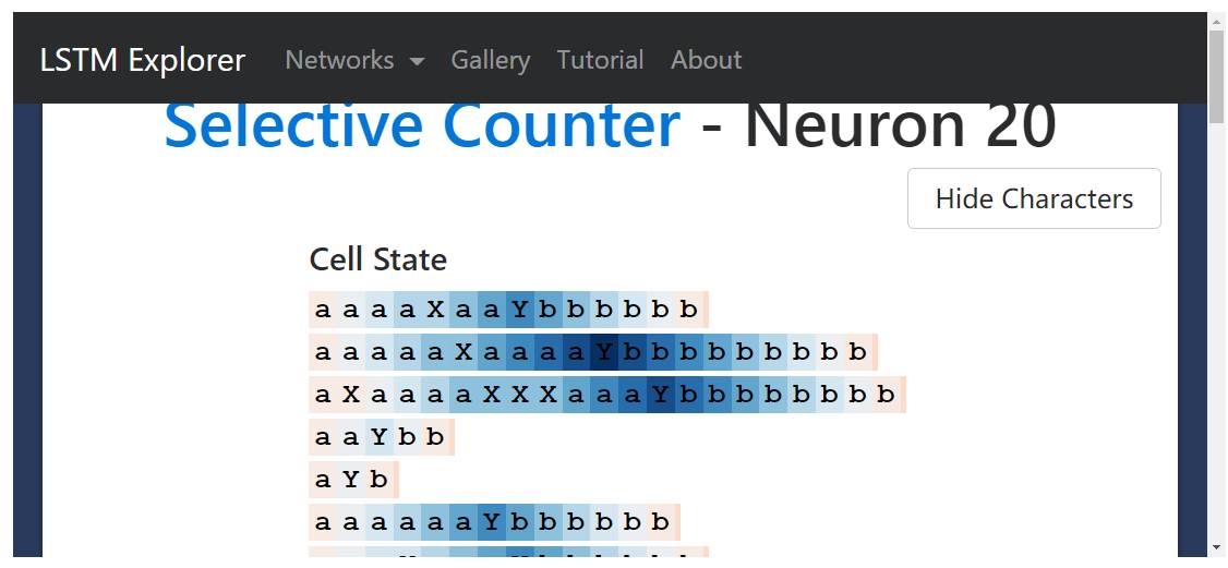
Check out the entire LSTM at this link (http://blog.echen.me/lstm-explorer/#/network?file=selective_counter) where we hope to see a counting neuron—a neuron that turns to 0 every time it sees an input gate X. And we did!

The above image shows neuron 20’s cell state. Its value keeps increasing until it encounters the separator Y, then it decreases until the end of the sequence—just like calculating a variable num_bs_left_to_print that increases with a’s and decreases with b’s.

If we look at its input gate, we will see that it indeed ignores the number of X’s:

However, interestingly, the candidate memory is fully activated on associated X’s—this shows why we need input gates. (However, if the input gate is not part of the model architecture, at least in this simple example, the network would still ignore the number of X’s in other ways.)

Now let’s look at neuron 10.

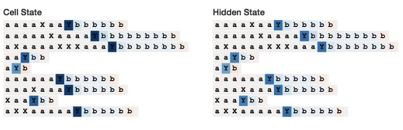
This neuron is interesting because it only activates when reading Y—yet it can still encode the number of a’s encountered in the sequence. (It might be hard to distinguish in the image, but when the number of a’s is the same, the color of Y is the same; even if not the same, the difference is within 0.1% of each other. You can see that in sequences with fewer a’s, the color of Y is lighter.) Perhaps other neurons will see neuron 10 as more relaxed.

Memory States

Next, I want to explore how LSTM remembers states. Similarly, I generated sequences of the following form:

AxxxxxxYa
BxxxxxxYb

(That is, either an “A” or “B”, followed by 1-10 x’s, then a separator “Y”, and finally ending with a lowercase starting character.) In this case, the network needs to remember whether it was a “state A” or a “state B”.

We hope to find a neuron that remembers the sequence starts with “A” and another that remembers it starts with “B”. We did.

For example, here is an “A” neuron that activates when reading “A” and continues to remember until it needs to generate the last letter. Note that the input gate ignores all x’s in the sequence.

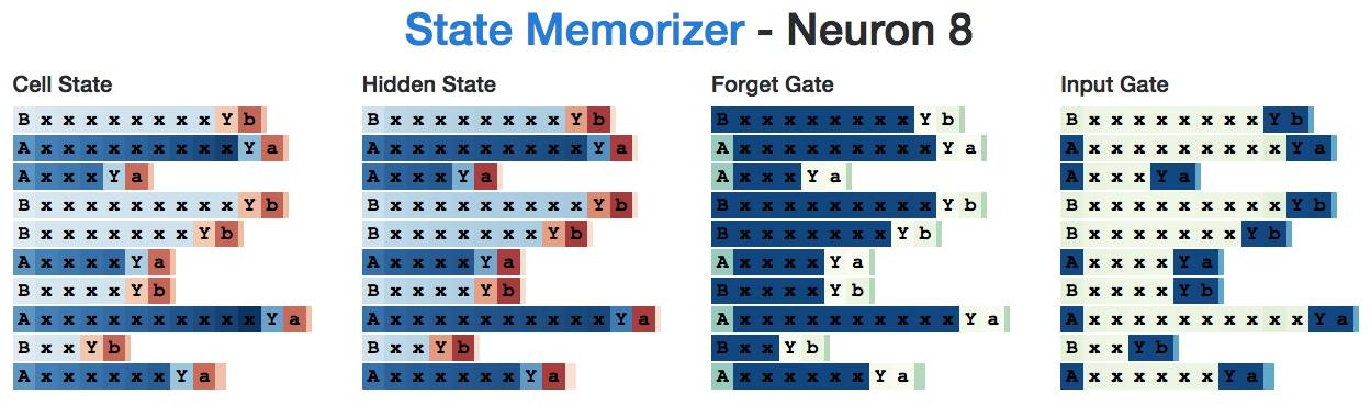
Below is the corresponding “B” neuron:

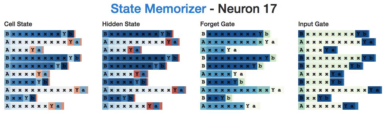
Interestingly, even before reading the separator “Y”, the knowledge about A and B is not needed, but the hidden state is present throughout all intermediate inputs. This seems a bit “inefficient” because the neuron is doing some double duty while counting x’s.

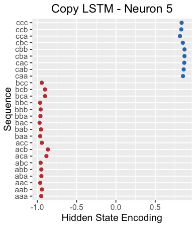
Copy Task

Finally, let’s look at how LSTM learns to copy information. (Recall that our Java LSTM learned to remember and copy an Apache license.)

For this copy task, I trained a small two-layer LSTM to generate sequences of the following form:

baaXbaa
abcXabc

(That is, a subsequence composed of characters a, b, c followed by a separator “X”, followed by the same subsequence again).

I was not sure what the “copy neuron” should look like, so to find neurons that could remember parts of the initial subsequence, I observed their hidden states when reading the separator X. As the neural network needs to encode the initial subsequence, its state should look different based on what it has learned.

For example, the following image shows the hidden state of neuron 5 when reading the separator “X”. This neuron clearly distinguishes sequences starting with “c” from those that do not.

Another example is the hidden state of neuron 20 when reading the separator “X”. It seems to select subsequences starting with “b”.

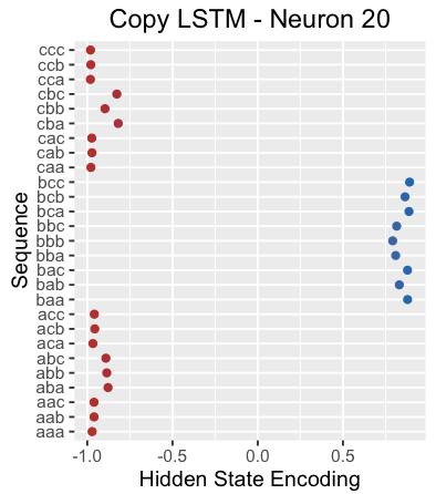
Interestingly, if we look at the cell state of neuron 20, it seems to capture all three subsequences.

Here is the overall cell state and hidden state of neuron 20 regarding the entire sequence. Note that its hidden state is off throughout the entire initial sequence (perhaps this is expected because its memory only needs to be kept passively at one point).

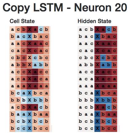
However, if we look a bit more closely, we find that as long as the next character is “b”, it is positive. So rather than the sequence starting with b, it is more like the sequence where the next character is b.

To my knowledge, this pattern exists throughout the network—all neurons seem to be predicting the next character rather than remembering the character that is currently in position. For example, neuron 5 seems to be a “next character” predictor.

I am not sure if this is the default type for LSTM when learning to copy information or what other types of copy mechanisms exist?

Extensions

Let’s review how you can explore LSTM yourself.

First, most problems we want to solve are sequential, so we should combine some past learnings into our model. But we already know that the hidden layers of neural networks encode their own information, so why not use these hidden layers as our memory to pass to the next step? This gives us Recurrent Neural Networks (RNN).

However, our behavior shows that we are unwilling to track knowledge; when we read a new political article, we do not immediately believe its content and combine it with our own beliefs about the world. We selectively save which information to keep, discard, and which information can be used to decide how to process the next news we read. Therefore, we want to learn to collect, update, and apply information—why not learn these things through their own mini neural networks? This gives us LSTM.

Now that we have gone through this process, we can also come up with our corrections:

• For example, perhaps you think it is foolish for LSTM to distinguish between long-term and working memory—why not use just one memory? Or perhaps you might discover that distinguishing between memory gates and saving gates is redundant—anything we forget should be replaced by new information, and vice versa. So now we have come up with a popular variant of LSTM, the Gated Recurrent Unit (GRU): https://arxiv.org/abs/1412.3555

• Or you might think that when deciding which information needs to be remembered, saved, or attended to, we should not rely solely on our working memory—why not use long-term memory at the same time? This leads to Peephole LSTM.

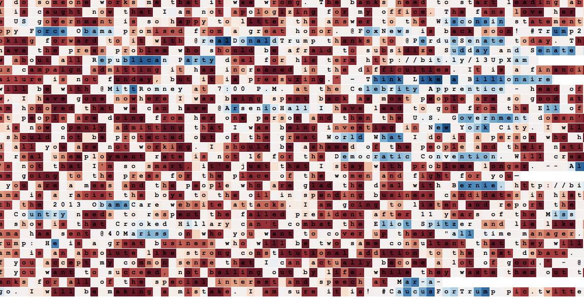
Let’s look at the final example, using a two-layer LSTM trained on Trump’s tweets. Although this is a large-scale dataset, this LSTM has been sufficient to learn many patterns.

For example, here is a neuron tracking positions within tags, URLs, and @mentions:

This is an appropriate noun detector (note that it is not simply focused on capitalized words):

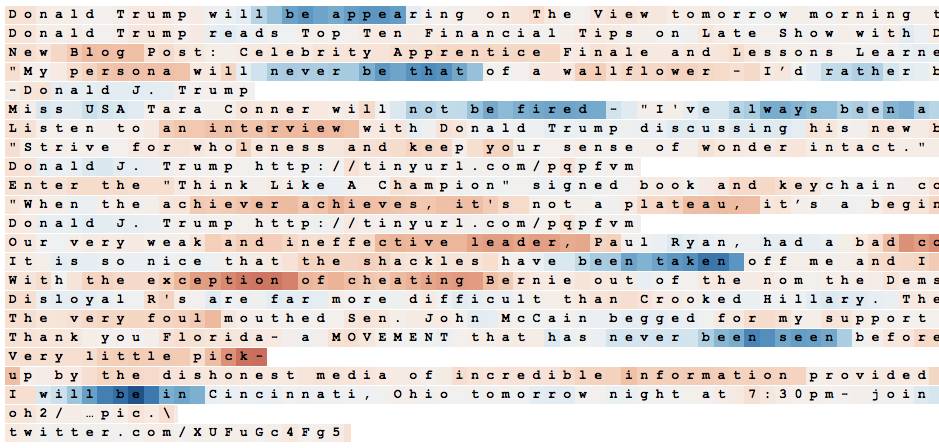
This is a detector for auxiliary verbs + “to be” (e.g., will be, I’ve always been, has never been):

This is a citation attribute:

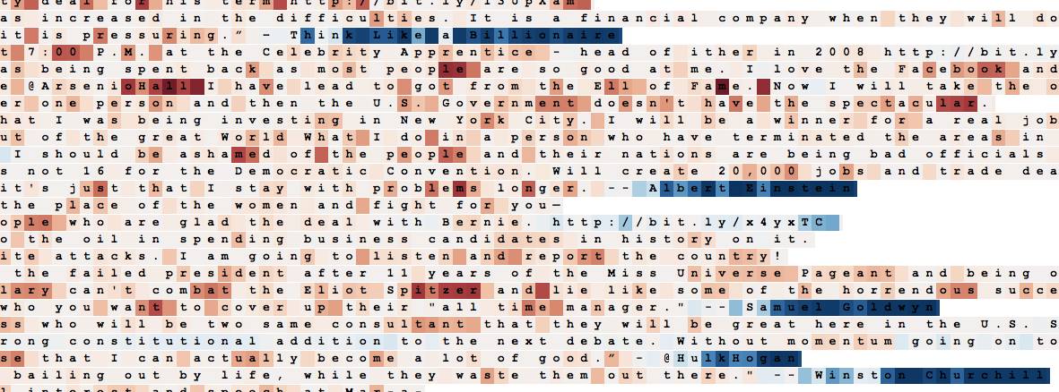
This is a MAGA and case-sensitive neuron:

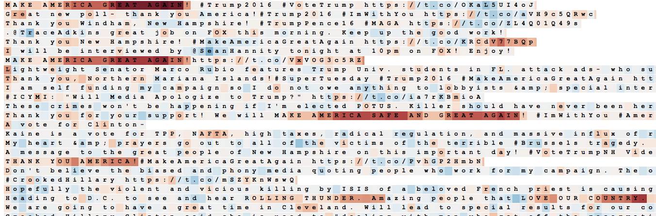
Here are some announcements generated by LSTM (okay, one of them is a real tweet, guess which one it is):

Unfortunately, LSTM only learned to write like a madman.

Original article link: http://blog.echen.me/2017/05/30/exploring-lstms/

This article is translated by Machine Heart, please contact this public account for authorization.

✄————————————————

Join Machine Heart (Full-time reporter/intern): [email protected]

Submissions or seeking coverage: [email protected]

Advertising & Business Cooperation: [email protected]

Click to read the original text and view the Machine Heart official website↓↓↓