Click on the above“Learn Visuals” to selectStar or “Top”
Heavyweight content, delivered first
Background Introduction
In common convolutional neural networks, sampling is almost everywhere, previously max pooling, now strided convolution.
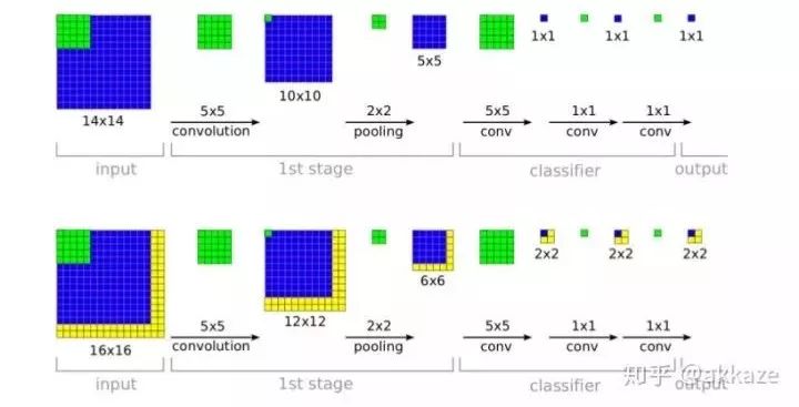
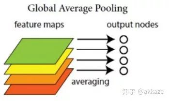
Taking the VGG network as an example, it uses quite a bit of max pooling.The input side is on the left (the bottom has padding, the top does not), and we can see that the network uses a lot of 2×2 pooling.Similarly, when doing semantic segmentation or object detection, we use quite a bit of upsampling, or transposed convolution.Typical FCN structure, note the red-highlighted deconvolution.Previously, we used FC in the last few layers of classification networks, but FC was later proven to have too many parameters and poor generalization, and was replaced by global average pooling, which first appeared in Network in Network.GAP directly aggregates each channel’s corresponding spatial features into a scalar.From then on, the paradigm of classification networks became (ReLU has been implicitly included in the conv and deconv),
Here we temporarily do not consider any shortcuts.
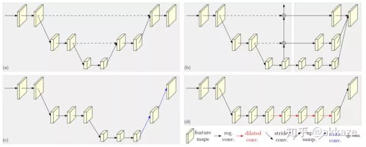
However, we must think, is downsampling and upsampling really necessary? Is it possible to remove them?Dilated Convolutions and Large Kernel Attempts
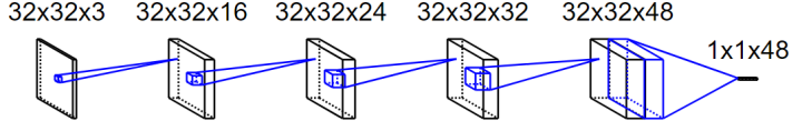
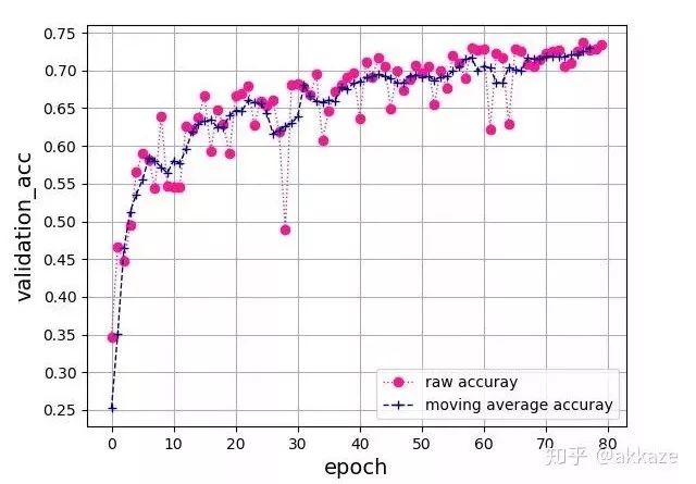
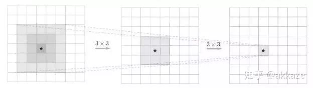
A very natural idea is that downsampling is only to reduce computational load and increase the receptive field. If there is no downsampling, to exponentially increase the receptive field, there are only two options: dilated convolutions and large kernel convolutions. So, the first step, in CIFAR10 classification, I tried removing downsampling, changing convolution to dilated convolution, and increasing the dilation rate respectively. The model structure is shown as follows,
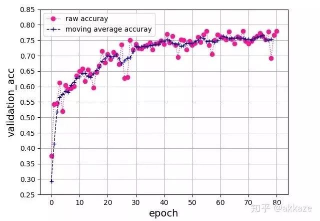
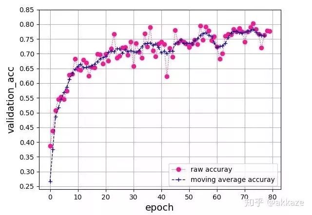
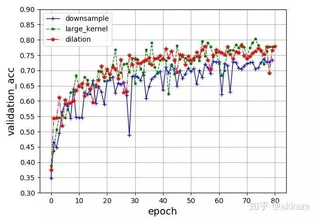
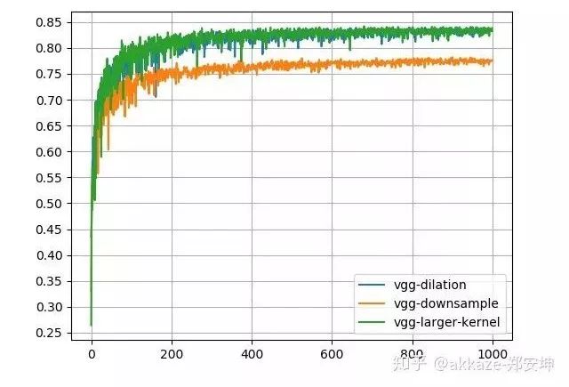
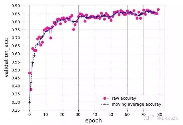
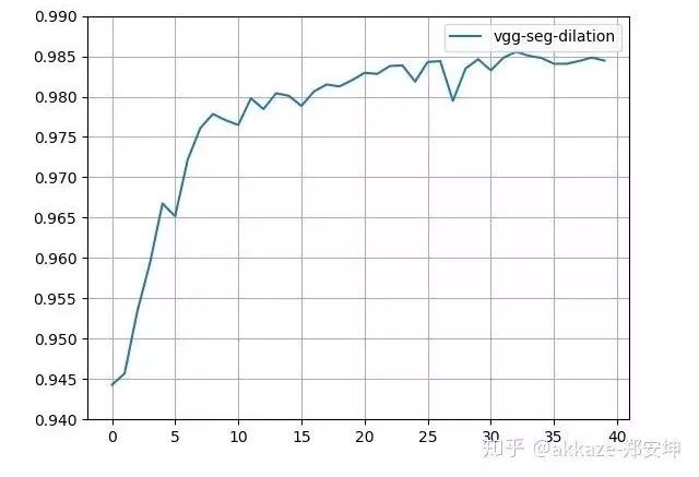
This network’s convolution structure, note that the last layer uses a spatial global average to flatten into a feature vector, followed by a 10-dimensional fully connected layer.This is a typical four-layer VGG structure, with dilation rates of 1, 2, 4, and 8 for each layer of convolution. After training for 80 epochs, the test accuracy curve is as follows,The accuracy of the four-layer VGG network, with convolution dilation rates of 1, 2, 4, and 8, has 25,474 trainable parameters.The final accuracy reached 76%, which is about the same accuracy that a VGG structured convolutional network with the same parameters can achieve.From another perspective, to expand the receptive field of the convolution, we can also directly increase the kernel size, maintaining the dilation rate at 1, while gradually increasing the kernel size of the convolution to 3, 5, 7, and 9. After training for 80 epochs, the accuracy curve is as follows,The four-layer VGG network, with convolution kernel sizes of 3, 5, 7, and 9, has 172,930 trainable parameters.Compared to the previous method of changing the dilation rate, the convergence process is quite consistent, with slight oscillation, but the final results are consistent, all around 76%. This indicates that the factors affecting the final accuracy are only the receptive field and the number of channels at each layer.To illustrate that downsampling does not improve performance, we will compare it with a network that includes downsampling. That is, without modifying any other parameters, using downsampling with stride set to 2 on the originally dilated convolutional layers, and training for 80 epochs, the convergence results are as follows,The four-layer VGG network, using stride 2 convolutions for downsampling at each layer, has 25,474 trainable parameters.The final convergence reached around 73%, which is about 3 points lower than the previous two experiments, indicating that the information loss from downsampling is indeed detrimental to CNN learning.Putting the results of the three parameter sets together for comparison can better illustrate the problem,Comparison results of the four-layer VGG network, where only the parameters of the convolutional layers differ, while all other parameters remain the same.For rigor, I will add the results of training for 1000 epochs,Results after training for 1000 epochs, showing a clear difference between the methods.To verify the universality of this idea, I used a ResNet18 structured network, replacing the convolutional layers that originally required downsampling with dilated convolutions that have increasing dilation rates. After training for 80 epochs, the final accuracy curve is shown as follows,Accuracy curve on ResNet18, obtained by changing the dilation rate of convolutional layers.Without any other parameter tuning, it finally converged to an accuracy of 87%.
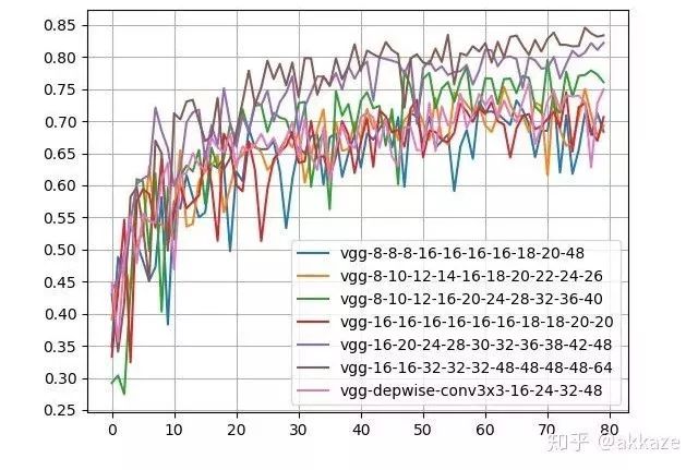
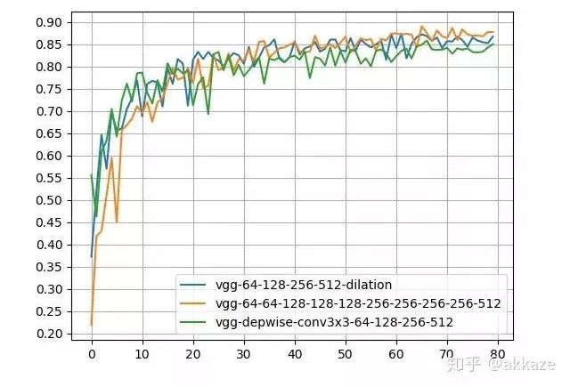
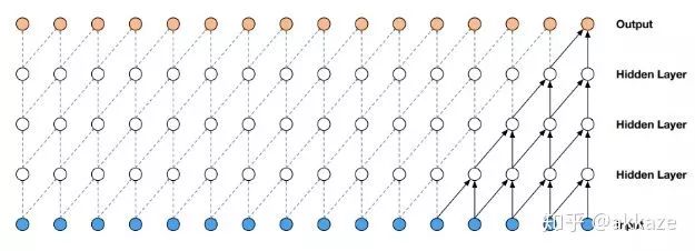
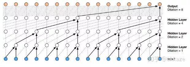
Small Kernel AttemptsWe know that the receptive field of a large convolution kernel can usually be achieved by stacking multiple small convolution kernels. VGGNet first discovered that a 5×5 convolution can be replaced by two 3×3 convolutions, greatly reducing the number of parameters.The receptive field of two 3×3 convolutions is the same as that of one 5×5 convolution, but with half the parameters.Similarly, a 7×7 convolution can be replaced by three 3×3 convolutions in series, and a 9×9 can be replaced by four 3×3 convolutions in series.To achieve the same receptive field as the previous four-layer convolution network, I designed a ten-layer network consisting only of 3×3 convolutions, with non-linear activations between each layer. Because the layer count increased significantly, I conducted several experiments to determine the number of channels in the intermediate layers. Meanwhile, to avoid significantly increasing the number of parameters, I inserted depthwise convolutions in between, maintaining the number of channels corresponding to the receptive field, while not increasing the parameter count too much. The training results are as follows,Experimental results, with the numbers indicating the number of channels for each layer.It can be seen that only three network structures outperform the previous design in terms of accuracy, and the parameters for these three networks are several times that of the previous design. The network using depthwise convolution did not significantly increase the number of parameters, but its accuracy was still slightly lower than the previous design.To illustrate the problem, I increased the number of channels in each layer, for example, changing from 16-32-48-64 to 64-128-256-512. Essentially, for this depth of network, the capacity is close to the upper limit, and the results are as follows,Results with increased channel numbers.It can be seen that the dilated convolution network still leads with fewer parameters compared to the depthwise convolution and mixed 3×3 convolution networks, with slightly lower accuracy than the 3×3 cascade network.This experiment shows that for CNNs, beyond depth, the receptive field and the number of channels corresponding to that receptive field truly determine the performance of the network.This is similar to the Wavenet in speech processing,General WavenetDilated WavenetWavenet uses dilated causal convolutions to reduce computational load. The original Wavenet performs well, but the computational load and parameter count grow exponentially.
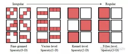
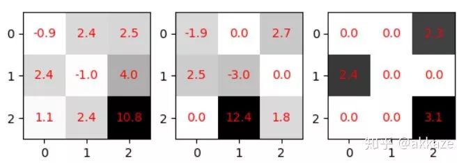
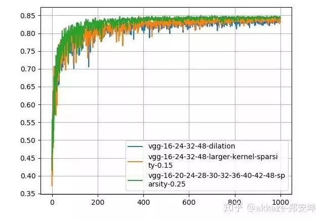
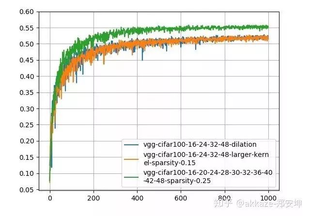
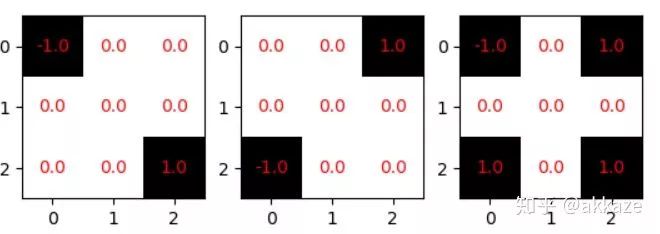
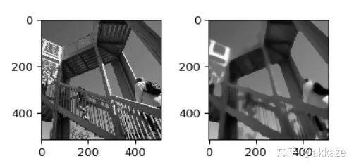
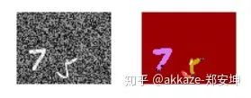
Thoughts on SparsityThe method of stacking small convolution kernels and using large convolution kernels incurs a huge parameter cost to achieve the same performance as dilated convolutions. Meanwhile, dilated convolutions are inherently sparse (most elements are 0), prompting us to consider whether sparsity can solve the problem of large parameters.Recent studies on CNN sparsity have been extensive. The general convolution sparsity is shown in the figure below, and it is noted that the convolution parameters of each layer are four-dimensional, specifically the number of input channels, the number of output channels, the convolution size in the x direction, and the convolution size in the y direction.Four types of different sparse convolutions; the leftmost is the least regular, while moving to the right, the dimensions become more regular, which is more favorable for hardware acceleration.What we commonly see is actually sparsity in the channel dimension, which reduces the number of channels and is the easiest to accelerate. However, a more meaningful sparsity, in my opinion, is the sparsity within the convolution kernels, as shown in the figure below,The leftmost has no sparsity, the middle has zero values (which means sparsity), and the rightmost has block sparsity of 1×2.This kind of sparsity can reduce the number of parameters (because zero values are meaningless), but because it is not conducive to engineering implementation, it currently does not show significant acceleration effects.Recent research indicates that most convolution kernels in CNNs are sparse, with over 50% being sparse, meaning that over 50% of the parameters are redundant. If redundant parameters can be removed, then large convolution kernels and multi-layer small convolution kernels can also demonstrate the decisive impact of receptive fields and the number of channels corresponding to those receptive fields on CNN performance, without adding extra model parameters.Although it is easy to predict, we will also prove the parameter redundancy of these two methods.The number of trainable parameters in a ten-layer 3×3 cascade network is 86,404, while the parameter count for a four-layer dilated convolution network is 25,474, and for a four-layer large convolution kernel network, it is 172,930. Using TensorFlow’s built-in sparsity feature, which can be found athttps://github.com/tensorflow/model-optimization, the principle is to set some elements of the convolution kernel to zero during training according to certain criteria, then fine-tune. For the ten-layer 3×3 cascade network, choosing a sparsity rate of 25% results in a post-sparsity parameter count of 21,601. For the large convolution kernel network, choosing a constant sparsity rate of 15% results in a post-sparsity parameter count of 25,940. Thus, after sparsity, their parameters are less than those of the dilated convolution network. To ensure that the network does not continue to converge, I trained for 1000 epochs, starting sparsity from the 200th epoch, and the training results after sparsity are as follows,It can be clearly seen that the performance of the sparsified 3×3 cascade network is the best, while it has the fewest parameters, followed by the large convolution kernel, at which point the performance of the dilated convolution is slightly lower.Maintaining the same parameters and sparsity, the results trained on CIFAR100 are as follows,At this point, the cascade 3×3 network’s performance has far surpassed the other two networks (for the appropriate baseline on CIFAR100, refer to some articles or blogs).Thoughts on Sparsity LimitsOur previous discussion essentially suggests that as long as a certain receptive field can be preserved, sparsity is feasible. However, one cannot help but wonder where the limits of sparsity lie. For a 3×3 convolution kernel, while preserving the receptive field, there must be at least two non-zero elements. But this leads to the convolution kernel degenerating from isotropic to anisotropic.The first two convolution kernels only have one directionality (diagonal direction), while the last one has two directionalities.Students who have studied linear algebra know that in a two-dimensional linear space, at least two basis vectors are needed to synthesize gradients in various directions. If the convolution kernel degenerates into the first two cases, its two-dimensional nature may be lost. However, as long as there are multiple convolution kernels with different directionalities in the same layer, that layer can still be isotropic, and directionality may also be an important descriptor of the receptive field. Regarding the directionality of the receptive field, an insight from experiments in the visual cortex is as follows,The distribution of receptive fields tuned to different directions in the human visual cortex.The Significance of Receptive Fields. Only large receptive fields can perceive larger objects. The receptive field, depth, and the number of channels together determine the performance of a certain layer in a CNN. A correct statement of CNN performance should indicate how deep the network is at a certain layer, what the receptive field is, and how many channels there are. Depth determines the network’s abstraction or learning ability, the receptive field determines how large an area the network can see at a certain layer, and the number of channels determines the amount of information at that layer. The receptive field and the number of channels can jointly represent the effective spatial and semantic information learned by the network at a certain layer.Additional Discussion on Max PoolingThis prompts us to think, is sampling really necessary? Of course, from an engineering perspective, sampling can greatly reduce the size of the feature map, thereby significantly reducing the computational load. However, this experiment shows that sampling does not help improve the performance of CNNs. Max pooling has a noise suppression effect, so it is useful, but max pooling can be implemented without downsampling, similar to classic median filtering.Typical median filtering, where the convolution kernel size is 20, noting that the output size does not change. Max pooling is similar to median filtering; both can be used to suppress noise.This also indicates that each convolution in a CNN encodes spatial correlations. Shallow features encode short-range correlations, while deeper convolutional layers encode longer-range spatial correlations. At a certain layer, there is no longer any statistically significant spatial correlation (this depends on the size of meaningful objects in the image). At this layer, global average pooling can be used to aggregate spatial features.Design of Segmentation NetworksBased on the previous classification network, removing the last global average pooling and fully connected layers, and replacing them with conv1x1 (many people know that the FC layer can be transformed into conv1x1, which was thought to be just an engineering trick, but it has essential connections), directly transforming into a segmentation network. The training results on my dataset M2NIST are as follows,Training results of the no-downsampling network on M2NIST (since the background area is large, an accuracy exceeding 94% is meaningful).Using the trained model for prediction, the visualized results are as follows:The left is the original image, and the right is the segmentation result, where a total of 10 digits need to be completely segmented.Subsequent Discussion on Possible Impacts on Network DesignIf there are no sampling layers, the paradigm of classification networks will be as follows:
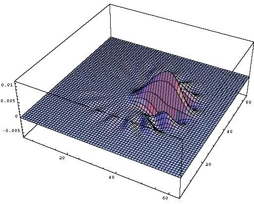
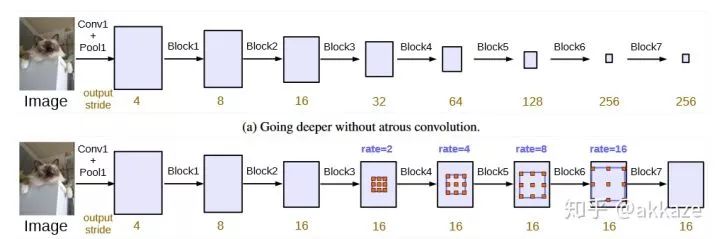
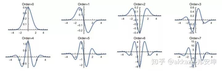
No more decoder phase, because at the decoder, upsampling is only to restore resolution. In the no-downsampling network structure, at the maximum receptive field, where global average pooling was previously added, softmax can be directly connected for pixel-level classification. More experiments are needed for this.In addition, in other networks, any part of the network can use no-downsampling subnetworks, such as the side networks of HRNet.No-downsampling networks can replace the original subnetworks that needed to restore resolution.Thoughts on Cross-Layer ConnectionsIf there is no sampling, then all feature maps will have the same resolution. Cross-layer connections will no longer distinguish between bottom-up and up-bottom; all cross-layer connections will essentially fuse features from different receptive fields (this is debatable; bottom-up should be fusing resolution, commonly used on the output side, while up-bottom should be fusing features from different receptive fields, commonly used on the feature extraction side. When there is no change in resolution, bottom-up is no longer needed).Possible Impacts on Object DetectionIf there is no change in resolution, then detection can completely branch into three branches at some receptive field in the deeper layers of the network, detecting large, medium, and small objects. This idea is similar to TridentNet.Thank you for the supplements in the comments. The dilated residual network has indeed been used in ResNet to handle classification and segmentation in a similar manner. I had not noticed this before, but even so, the last layer of DRN still has a sampling process, while this article attempts to directly construct a network without any sampling. Moreover, my article does not intend to focus on dilated convolutions; the earlier parts of my article aim to clarify whether sampling is necessary and attempt to illustrate the dialectical relationship between receptive fields, depth, and channel counts, as well as the essence of the directionality of receptive fields and convolution sparsity. Recently, research on sparse convolutions has actually been increasing; those interested can refer to arXiv for more information, and I won’t list them all here.Please realize that dilated convolution is not necessary; a larger kernel size convolution can replace it, but this will inevitably introduce more parameters, potentially leading to overfitting. Of course, this can be addressed using sparsity methods, but sparse convolutions are currently not suitable for engineering because they are not efficient.Similar ideas first appeared in the DeepLab-related paper “Rethinking Atrous Convolution for Semantic Image Segmentation” (https://arxiv.org/abs/1706.05587), where atrous convolution primarily removes downsampling operations in the last few layers of the network and corresponding upsampling operations of the filters to extract more compact features without adding new learning parameters.Image from the paper, designed in a serial manner, duplicating the last block of ResNet, such as block4, and cascading the copied blocks in a serial manner.To summarize this article.Although it is detrimental to acceleration, convolutional kernels should inherently be sparse. Downsampling loses resolution, which will inevitably lead to a loss of accuracy. Beyond depth, only the receptive field and the corresponding number of channels are most important.Mathematical Essence of Thought (this part can be ignored as needed, I plan to discuss it separately in the future)The last small section has been expanded into another articlehttps://zhuanlan.zhihu.com/p/99193115, this article’s other function is to make it easier for mathematicians to analyze CNNs without having to model downsampling, only needing to prove that the sparsity of convolutional kernels can model image recognition. Moreover, with the removal of sampling, convolution becomes convolution in continuous space (simultaneously, activation functions can also be softened), and the kernel size can be described using the function support space (similar to the effective radius of the Gaussian kernel). The image below is the Gaussian kernel function under different images,In short, CNN is a neural network that uses convolutions to map from two-dimensional functional spaces to two-dimensional functional spaces.In one dimension, this is equivalent to mapping a bounded function f on (-1, 1) to a bounded function g,Why use convolutions? It is well-known that convolutions are the simplest such functional.Moreover, it has many good properties, the most important of which is that convolutions have translational invariance,It also has scale invariance,It has associativity and commutativity.So for any operator , the purpose of CNN is to find such a .However, finding this directly is not easy, so we use a series of convolutions to approximate it, where is the non-linear activation function.Then the strategy of CNN is obvious: to approximate any functional using a set of convolutions (note that at this point, the scale invariance is broken by non-linear activation).Why use small convolution kernels to approximate Dirac and Gaussian functions?We know that the Dirac functionIt is a generalized function, meaning it is not a function in the ordinary sense. When the effective radius of the Gaussian kernel function approaches zero, it becomes the Dirac function.Its convolution has the following properties:This can be seen as a 1×1 convolution,Its n-th derivative has the following properties:In other words, convolving with its n-th derivative yields its own n-th derivative.This function cannot be realized in practice, but let’s look at the Gaussian function and see what its derivatives look like.The first seven derivatives of the Gaussian function, including the original function, show an astonishing consistency in effective radius.It can be seen that these functions have remarkably consistent effective radii. If these functions are used, theoretically, any differential operator can be approximated using convolutions, and differential operators are very well-behaved linear operators.So, why use small convolution kernels? Because only when the effective radius of the Gaussian function approaches zero can it approximate the Dirac function, and its derivatives can approximate the derivatives of the Dirac function.(The significance of small convolution kernels is debatable; here is another way of thinking: because images are not ordinary functions, convolutions become multiplication in frequency space. Small convolution kernels are more likely to produce high frequencies (analogous to Gaussian kernel functions), so convolutions are more likely to amplify high-frequency information (in fact, this does not completely contradict the above explanation), making high-frequency information less likely to be erased by non-linear activation functions. High-frequency information is very important for images, such as edges and corners).The significance of slightly larger convolution kernelsIn fact, the Gaussian kernel has another property: after applying the Gaussian kernel (equivalent to Gaussian averaging), the n-th derivative is equivalent to convolving with the n-th derivative of the Gaussian kernel, meaning that,At the same time, the Gaussian kernel has the following properties:Thus, we have the Gaussian kernel as a basis vector, withThus, solving this is equivalent to solving a series of linear coefficients , please correspond to the kernel size.Then, the significance of slightly larger convolution kernels is to transform the differential operator in the space after Gaussian averaging. Moreover, the larger the kernel, the stronger the smoothing effect.In the image domain, due to the discretization of computer and information theory, we use sampling and quantization to process it, thereby reducing computational load.Please continue to pay attention to the source code GitHub repository of this article(https://github.com/akkaze/cnn-without-any-downsampling)Author: Zhihu – Akkaze – Zheng AnkunAddress: https://www.zhihu.com/people/kkk-37-60Download 1: OpenCV-Contrib Extension Module Chinese Version TutorialReply in the background of “Learn Visuals” public account:Chinese Tutorial for Extension Modules, to download the first Chinese version of the OpenCV extension module tutorial on the internet, covering installation of extension modules, SFM algorithms, stereo vision, object tracking, biological vision, super-resolution processing and more than twenty chapters.Download 2: Python Visual Practical Projects 52 LecturesReply in the background of ““Learn Visuals” public account: Python Visual Practical Projects, to download 31 visual practical projects including image segmentation, mask detection, lane line detection, vehicle counting, eyeliner addition, license plate recognition, character recognition, emotion detection, text content extraction, face recognition, etc., to help quickly learn computer vision.Download 3: OpenCV Practical Projects 20 LecturesReply in the background of ““Learn Visuals” public account: OpenCV Practical Projects 20 Lectures, to download 20 practical projects based on OpenCV to advance OpenCV learning.
Group chat
Welcome to join the public account reader group to communicate with peers. Currently, there are WeChat groups on SLAM, three-dimensional vision, sensors, autonomous driving, computational photography, detection, segmentation, recognition, medical imaging, GAN, algorithm competitions etc. (which will gradually be subdivided in the future). Please scan the WeChat number below to join the group, with a note: “Nickname + School/Company + Research Direction”, for example: “Zhang San + Shanghai Jiao Tong University + Visual SLAM”. Please follow the format for notes; otherwise, it will not be approved. After successfully adding, invitations will be sent to the relevant WeChat groups based on research direction. Please do not send advertisements in the group, or you will be removed from the group. Thank you for your understanding.

 under different
  images,
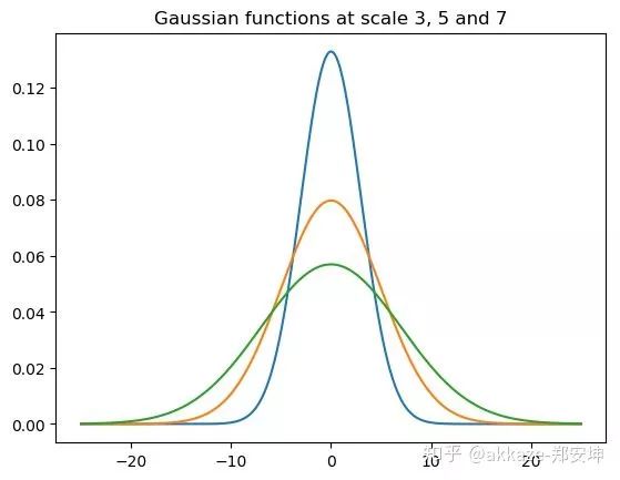


 , the purpose of CNN is to find such a
  .
.
 is the non-linear activation function.


 , please correspond
  to the kernel size.