
Author: Tianqi Chen, graduated from Shanghai Jiao Tong University ACM class, currently studying at the University of Washington, engaged in large-scale machine learning research.
Note: truth4sex
1. Introduction
At the invitation of @Longxing Biaoju, I am writing this article. As a very effective machine learning method, Boosted Trees are one of the most commonly used algorithms in data mining and machine learning. Due to its effectiveness and insensitivity to input requirements, it is often an essential tool for statisticians and data scientists, and it is also the most commonly used tool by Kaggle competition champions. Lastly, due to its good performance and low computational complexity, it has a wide range of applications in the industry.
2. Synonyms for Boosted Trees
At this point, some may wonder why they have not heard of this name. This is because Boosted Trees have various aliases, such as GBDT, GBRT (Gradient Boosted Regression Tree), MART1, and LambdaMART, which is also a variant of boosted trees. There is a lot of material online introducing Boosted Trees, but most of it is based on the early article by Friedman, “Greedy Function Approximation: A Gradient Boosting Machine.” Personally, I think this is not the best or most general way to introduce Boosted Trees. Moreover, there are not many introductions outside of this perspective. This article is my personal summary of Boosted Trees and algorithms of the gradient boosting class, much of which is derived from a lecture note2 I used while being a TA for machine learning at UW.
3. Logical Components of Supervised Learning Algorithms
To discuss Boosted Trees, we must first talk about supervised learning. In supervised learning, there are several logically important components3, which can be roughly divided into: model, parameters, and objective function.
i. Model and Parameters
The model refers to how to predict the output yi given the input xi. Common models like linear models (including linear regression and logistic regression) use a linear combination for prediction.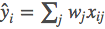 In fact, the prediction y here can have different interpretations; for instance, we can use it as the output for a regression target, or apply a sigmoid transformation to obtain probabilities, or as a ranking metric, etc. A linear model can be applied in regression, classification, or ranking scenarios depending on how y is interpreted (and the corresponding objective function designed). Parameters refer to what we need to learn; in a linear model, the parameters refer to our linear coefficients w.
ii. Objective Function: Loss + Regularization
The model and parameters specify how we make predictions given input, but do not tell us how to find good parameters; this is where the objective function comes into play. A general objective function consists of the following two components:

Common error functions include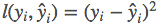 , such as squared error
 logistic error function
 , etc. Common regularization terms for linear models include L2 regularization and L1 regularization. The design of the objective function stems from an important concept in statistical learning called Bias-Variance Tradeoff4. A more intuitive understanding is that Bias can be understood as the error obtained from training the best model when we have infinitely many data points. Variance, on the other hand, arises from the randomness of having only a finite amount of data. The objective error function encourages our model to fit the training data as closely as possible, which tends to result in a model with lower bias. The regularization term, however, encourages simpler models. When the model is simpler, the randomness in the results fitted from the finite data is smaller, making it less prone to overfitting, thus stabilizing the final model’s predictions.
iii. Optimization Algorithm
Having discussed the basic concepts of supervised learning, why is this important? It is because these components contain the main elements of machine learning and provide an effective way to modularize the design of machine learning tools. In fact, aside from these components, there is also an optimization algorithm, which addresses how to learn given an objective function. The reason I have not discussed optimization algorithms is that they are often the “machine learning part” that everyone is familiar with. However, sometimes we only know about “optimization algorithms” without carefully considering the design of the objective function. A common example is decision tree learning; everyone knows that the algorithm optimizes the Gini index at each step and then prunes, but does not consider what the later objective is.
4. Boosted Tree
i. Base Learner: Classification and Regression Trees (CART)
Returning to the topic of Boosted Trees, we will start discussing from these aspects, beginning with the model. The most basic component of Boosted Trees is called a regression tree, also known as CART5.
The above is an example of a CART. CART allocates inputs to various leaf nodes based on the attributes of the input, with each leaf node corresponding to a real-valued score. The example above predicts whether a person will like computer games; you can interpret the score of the leaf as the likelihood of that person enjoying computer games. Some may ask about its relationship with decision trees; we can simply understand it as an extension of decision trees. From simple class labels to scores, we can do many things, such as probability predictions, and ranking.
ii. Tree Ensemble
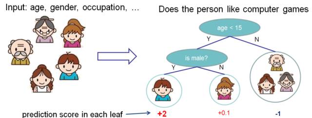
A single CART is often too simple to make effective predictions, hence a more powerful model called tree ensemble is used.
In the example above, we use two trees to make predictions. The predicted result for each sample is the sum of the predicted scores from each tree. At this point, we have introduced our model. Now the question arises: what is the relationship between common random forests and boosted trees and tree ensembles? If you think carefully, you will find that both RF and boosted trees are tree ensembles, but the methods for constructing (learning) the model parameters differ. The second question is: what are the “parameters” in this model? In tree ensembles, parameters correspond to the structure of the trees and the predicted scores at each leaf node.
The final question is, of course, how to learn these parameters. For this part, the answer may vary widely, but the standard answer is always the same: define a reasonable objective function and then attempt to optimize that objective function. I would like to emphasize that decision tree learning is often filled with heuristics, such as optimizing the Gini index first and then pruning, or restricting the maximum depth, etc. In fact, these heuristics often imply an underlying objective function, and understanding the objective function itself also aids in designing learning algorithms, which will be elaborated on later.
For tree ensembles, we can more rigorously express our model as:

where each f is a function within the function space6 (F), and F corresponds to the set of all regression trees. The designed objective function must also adhere to the earlier main principles, containing two parts:

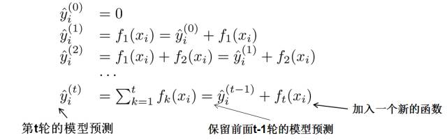
iii. Model Learning: Additive Training
The first part is the training error, which includes familiar metrics like squared error, logistic loss, etc. The second part is the sum of the complexities of each tree, which will be discussed further later. Since our parameters can be considered to reside in a function space, we cannot use traditional algorithms like SGD to learn our model; instead, we will use a method called additive training (additionally, in my personal understanding, boosting refers to additive training). Each time, we keep the original model unchanged and add a new function f to our model.
Now there is still one question: how do we choose which f to add each round? The answer is straightforward: select an f that maximally reduces our objective function8.
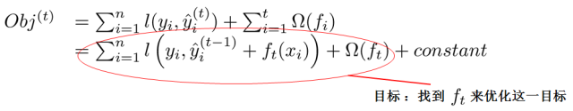
This formula may be a bit abstract; we can consider the case when ll is squared error. In this case, our objective can be expressed as the following quadratic function9:
More generally, for cases other than squared error, we will use a Taylor expansion approximation to define an approximate objective function to facilitate our calculations for this step.
After removing the constant term, we find a more unified objective function. This objective function has a very obvious characteristic: it only depends on the first and second derivatives of each data point in the error function10. Some may ask why this material seems more difficult to understand than what we previously learned about decision tree learning. Why go through so much effort to derive?
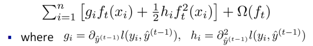
The reason is that this allows us to clearly understand the overall objective and derive step by step how to conduct tree learning. This abstract form is also very helpful for implementing machine learning tools. Traditional GBDT may be understood as optimizing the residuals, but this form encompasses all differentiable objective functions. This means that with this form, the code we write can be used to solve various problems including regression, classification, and ranking, and the formal derivation makes machine learning tools more general.
iv. Tree Complexity
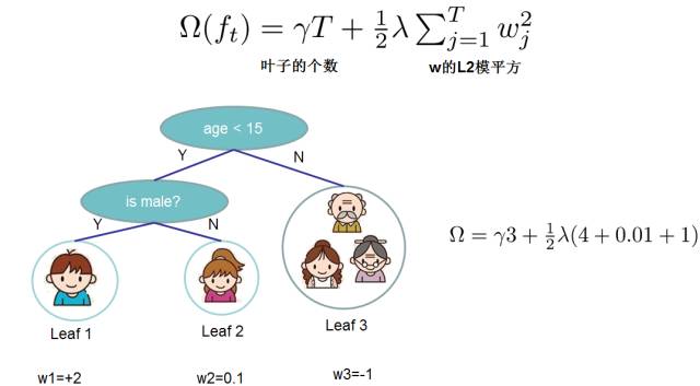
So far, we have discussed the training error part of the objective function. Next, we will discuss how to define tree complexity. We first refine the definition of f, breaking the tree down into its structural part q and the leaf weight part w. The following diagram provides a specific example. The structural function q maps inputs to the index numbers of the leaves, while w specifies the score corresponding to each index.
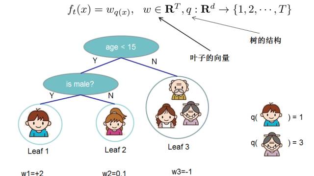
Once we have provided the above definition, we can define the complexity of a tree as follows. This complexity includes the number of nodes in a tree and the squared L2 norm of the output scores at each leaf node. Of course, this is not the only way to define it, but this definition typically yields trees with good performance. The diagram below also provides an example of complexity calculation.
v. Key Steps
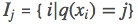
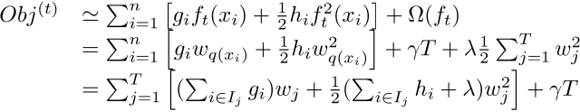
The next step is the most crucial11, under this new definition, we can rewrite the objective function as follows, where I is defined as the sample set on each leaf:
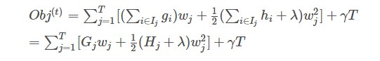
This objective consists of T mutually independent univariate quadratic functions. We can define:

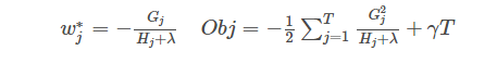
Then this objective function can be further rewritten in the following form, assuming we already know the tree structure q, we can use this objective function to solve for the best w, and the best w corresponds to the maximum gain of the objective function.
The results correspond as follows: the left is the best w, and the right is the value of the objective function corresponding to this w. At this point, you may find this derivation slightly complex. In fact, it only involves how to find the minimum of a univariate quadratic function12. If you feel you do not understand, it is worth taking some time to ponder.
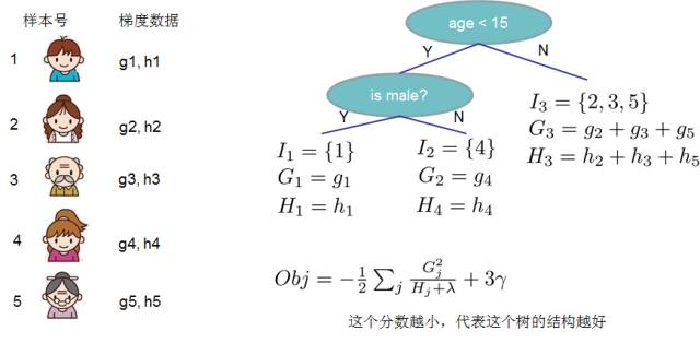
vi. Example of Scoring Function Calculation
Obj represents how much we can reduce the objective when we specify a tree structure. We can refer to this as the structure score. You can think of this as a more general scoring function for tree structures, similar to the Gini index. Below is a specific example of scoring function calculation.
vii. Greedy Method for Enumerating All Different Tree Structures
Thus our algorithm is quite simple; we continuously enumerate different tree structures, using this scoring function to find an optimal tree structure to add to our model, and repeat this operation. However, enumerating all tree structures is not feasible, so the common method is the greedy approach, where we attempt to add a split to existing leaves each time. For a specific splitting scheme, the gain can be calculated using the formula below.
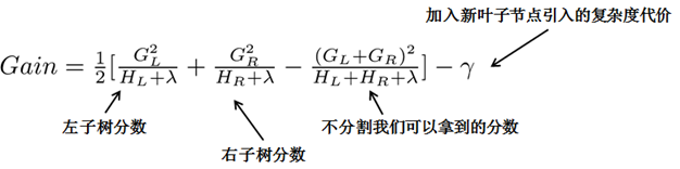
For each expansion, we still need to enumerate all possible splits. How do we efficiently enumerate all splits? I assume we want to enumerate all conditions of the form x<a; for a specific split a, we need to calculate the sums of gradients on the left and right sides.
We can observe that for all a, we only need to perform a single left-to-right scan to enumerate the gradient sums GL and GR for all splits. Then we can use the above formula to calculate the score for each splitting scheme.
Observing this objective function, you will notice another important aspect: introducing a split does not necessarily improve the situation, as we have a penalty term for introducing new leaves. Optimizing this objective corresponds to tree pruning; when the gain from the introduced split is below a threshold, we can prune that split. You may find that when we formally derive the objective, strategies like calculating scores and pruning naturally emerge, rather than being heuristic operations.
At this point, the article is nearing its conclusion. Although it is somewhat lengthy, I hope it is helpful to everyone. This article introduces how to derive the learning of Boosted Trees through a method of optimizing the objective function. With such a general derivation, the resulting algorithm can be directly applied to various application scenarios, including regression, classification, and ranking.
5. Conclusion: XGBoost
All the derivations and techniques discussed in this article guide the design of XGBoost https://github.com/dmlc/xgboost. XGBoost is a tool for large-scale parallel boosted trees, and it is currently the fastest and best open-source boosted tree toolkit, being over ten times faster than common toolkits. In the field of data science, many Kaggle competitors use it for data mining competitions, including winning solutions for more than two Kaggle competitions. In terms of industrial scale, the distributed version of XGBoost has wide portability, supporting operation on platforms such as YARN, MPI, and Sungrid Engine, while retaining various optimizations from the single-machine parallel version, making it well-suited for solving industrial-scale problems. Interested students can try it out and are welcome to contribute code.
Annotations and Links:
1: Multiple Additive Regression Trees, Jerry Friedman, KDD 2002 Innovation Award http://www.sigkdd.org/node/362
2: Introduction to Boosted Trees, Tianqi Chen, 2014 http://homes.cs.washington.edu/~tqchen/pdf/BoostedTree.pdf
3: Principles of Data Mining, David Hand et al, 2001. Chapter 1.5 Components of Data Mining Algorithms, decomposing data mining algorithms into four components: 1) Model structure (functional form, such as linear models), 2) Scoring function (assessing the quality of model fit to data, such as likelihood functions, squared error, misclassification rate), 3) Optimization and search methods (optimization of scoring functions and solving model parameters), 4) Data management strategies (efficient access to data during optimization and search).
4: In probability and statistics, the criteria for selecting parameter estimators are three: 1) Unbiasedness (the mean of the parameter estimator equals the true value of the parameter), 2) Efficiency (the smaller the variance of the parameter estimator, the better), 3) Consistency (as the sample size gradually increases from a finite number to infinite, the parameter estimator converges in probability to the true value of the parameter). “Probability Theory and Mathematical Statistics”, Gao Zuxin et al, 1999, Section 7.3 Criteria for Estimating Parameters
5: Breiman, L., Friedman, J., Stone, C. J., & Olshen, R. A. (1984). Classification and Regression Trees. CRC Press. Breiman received the KDD 2005 Innovation Award
6: F is the functional space, or hypothesis space; f is a function, or hypothesis. Here, the ensemble consists of K components/base learners, and their combination is an unweighted sum. NOTE: [In general boosting (like AdaBoost), f is added with weights because those weights are naturally absorbed into the leaf weights.] by Chen Tianqi
7: Friedman et al. (Friedman, J., Hastie, T., & Tibshirani, R. (2000). Additive Logistic Regression: A Statistical View of Boosting (with discussion and a rejoinder by the authors). The Annals of Statistics, 28(2), 337-407.) provided a statistical interpretation for the boosting ensemble learning paradigm in 2000, namely additive logistic regression. However, they could not fully explain the overfitting resistance of the AdaBoost algorithm. Nanjing University’s Zhou Zhihua et al. http://www.slideshare.net/hustwj/ccl2014-keynote addressed this issue more comprehensively from the perspective of statistical learning theory’s margin distribution.
8: This idea is the basis of boosting algorithms like AdaBoost: serially generating a series of base learners, such that each current base learner focuses on the data samples where all previous learners made errors, thus achieving improvement.
9: Note that the optimization search variable is f (i.e., searching for the current base learner f), so all terms not related to f are absorbed into the const, such as the current error loss.
10: 1). The first coefficient g and the second coefficient 1/2*h 2) of the variable to be optimized f. The error function with respect to is differentiated, involving the previous t−1 base learners, as they determine the current prediction result.
11: Since each data point falls into exactly one leaf node, we can group n data points by leaf, similar to combining like terms; two data points are of the same class if they fall into the same leaf, i.e., the indicator variable set Ij here.
12: The variable is wj, and the quadratic function with respect to it is: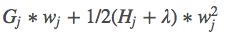 , and this function is differentiated with respect to the variable wj and set to zero, yielding the expression.
This article was first published on: I Love Computer Science
Original title: XGBoost and Boosted Trees