Detailed Derivation of XGBoost Explained

– What is the basis for tree node splitting in XGBoost?

– How is the weight of tree nodes calculated?

– What improvements has XGBoost made to prevent overfitting?

Those reading this article are likely familiar with XGBoost. Indeed, XGBoost is not only a powerful tool in major data science competitions but is also widely used by many companies in practical work.

As competition for algorithm positions becomes increasingly fierce, the difficulty of interviews is evident to all. Simply memorizing a few common interview questions is far from sufficient; interviewers often dig deeper, focusing on candidates’ depth of understanding of the model. Therefore, with XGBoost, you need to understand not just how it works but also why it works.

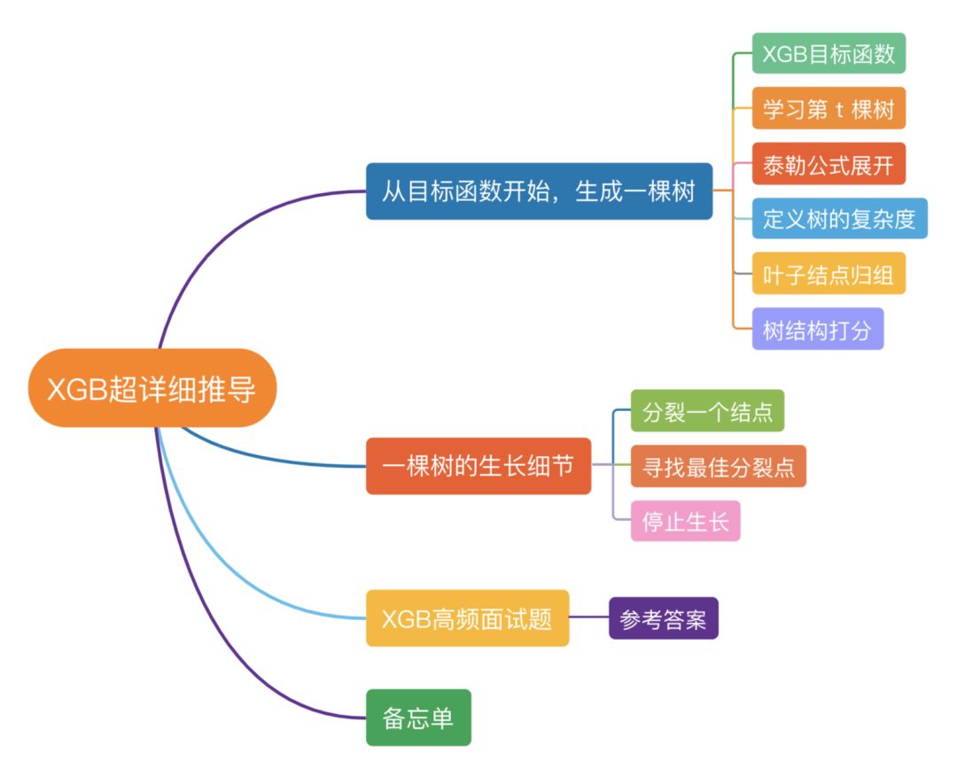
This article focuses on the derivation process of XGBoost. At the end, I will present 10 interview questions to test everyone, and finally, I have prepared a “XGBoost Derivation Cheat Sheet” to help you better grasp the entire derivation process.

Structure of This Article

Starting from the “Objective Function” to Generate a Tree

1. XGBoost Objective Function

The objective function of XGBoost consists of training loss and regularization term, defined as follows:

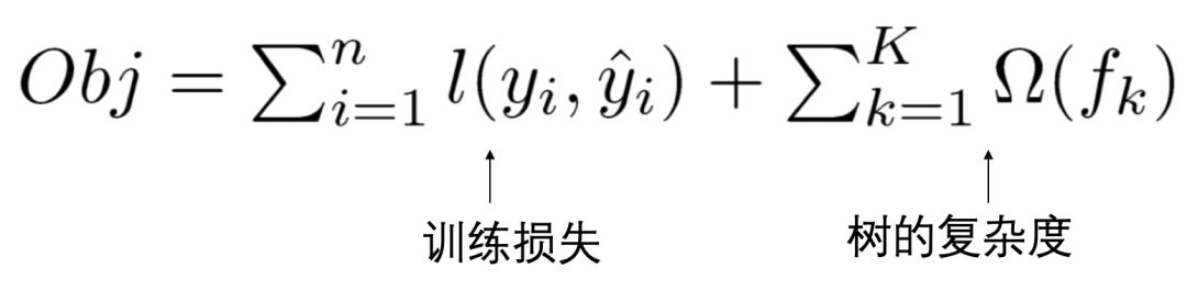
Variable Explanation:

(1) l represents the loss function, common loss functions include: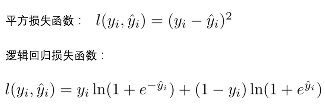

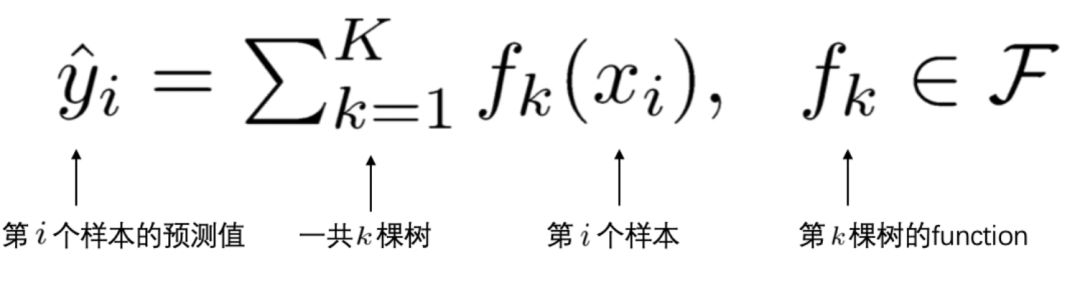
(2) yi’ is the predicted value of the ith sample xi. Since XGBoost is an additive model, the predicted score is the cumulative sum of the scores from each tree.

(3) The complexity of all k trees is summed and added to the objective function as a regularization term to prevent overfitting.

2. Learning the t-th Tree

As mentioned in [1], XGBoost is an additive model. Assuming the tree model we want to train in the t-th iteration is ft(), we have:

Substituting this into the objective function Obj in [1], we can obtain:

Note that in the above equation, there is only one variable, which is the t-th tree:

The rest are known quantities or can be calculated from known quantities (be sure to understand this!).

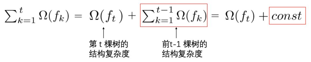
Careful students may notice that we have split the regularization term here. Since the structure of the first t-1 trees is already determined, the sum of the complexities of the first t-1 trees can be represented as a constant:

3. Taylor Expansion

First, let’s briefly recall the Taylor expansion.

The Taylor formula approximates a function f(x) that has n derivatives at x = x0 using an n-degree polynomial about (x-x0).

The second-order expansion form of the Taylor formula is as follows:

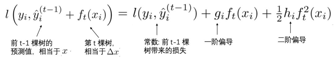
Returning to our problem, f(x) corresponds to our loss function l, x corresponds to the predicted values of the first t-1 trees, and Δx corresponds to the t-th tree we are training.

First, we define the first-order partial derivative and second-order partial derivative of the loss function l with respect to y'(t-1):

Thus, our loss function can be transformed into the following form (showing the correspondence with x and Δx in the Taylor formula).

Substituting the above second-order expansion into the objective function Obj in [2], we can obtain an approximation of the objective function Obj:

Removing all constant terms, we obtain the objective function:

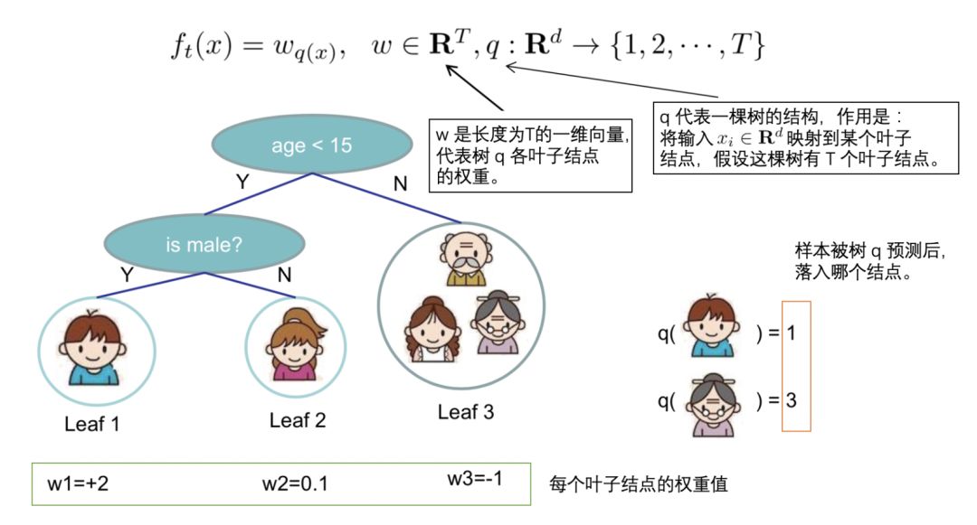
4. Defining a Tree

We redefine a tree, which includes two parts:

Weight vector of leaf nodes ω;
Mapping relationship from instances to leaf nodes q (essentially the branching structure of the tree);

The expression of a tree is defined as follows:

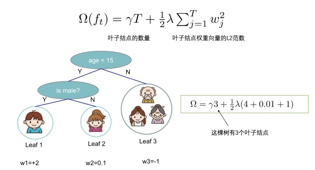
5. Defining Tree Complexity

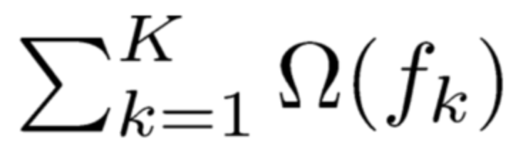
We define the complexity Ω of a tree, which consists of two parts:

Number of leaf nodes;
L2 norm of the weight vector of leaf nodes;

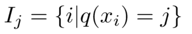
6. Grouping Leaf Nodes

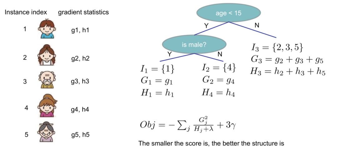
We group all samples xi belonging to the j-th leaf node into a leaf node sample set, mathematically represented as:

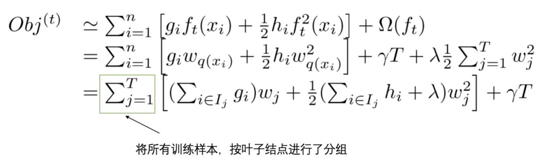
Then, we substitute the definitions of a tree and its complexity from [4] and [5] into the Taylor-expanded objective function Obj in [3], with the specific derivation as follows:

To further simplify this expression, we make the following definitions:

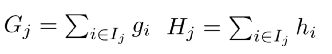
Meaning as follows:

Gj: The sum of the <span>first-order partial derivatives</span> of the samples contained in leaf node j, is a constant;
Hj: The sum of the <span>second-order partial derivatives</span> of the samples contained in leaf node j, is a constant;

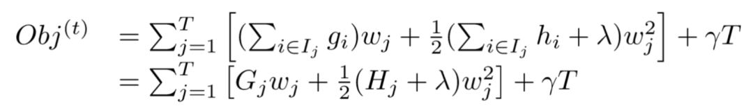
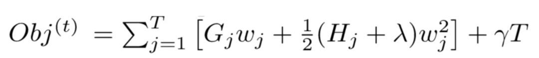
Substituting Gj and Hj into the objective function Obj, we obtain our final objective function (note that at this point, the only variable left in the expression is the weight vector W of the t-th tree):

7. Scoring Tree Structure

Recall some knowledge from high school mathematics. Suppose we have a quadratic function in one variable, in the following form:

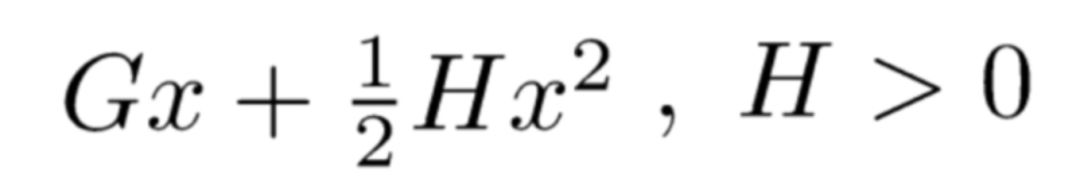
We can easily find the extremum point using the extremum formula for quadratic functions:

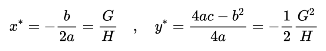
Now, returning to our objective function Obj, how do we find its extremum?

First, let’s analyze the above expression:

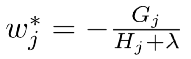
For each leaf node j, we can extract it from the objective function Obj:

As mentioned in [6], Gj and Hj can be calculated with respect to the t-th tree. Thus, this expression is a univariate quadratic function that contains only one variable, the weight wj of the leaf node.

Further analyzing the objective function Obj, we can find that the objective sub-expressions for each leaf node are independent of each other, meaning that when each leaf node’s sub-expression reaches its extremum, the entire objective function Obj also reaches its extremum.

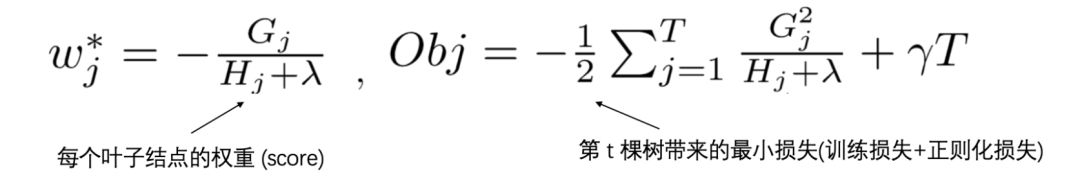
Now, assuming the structure of the tree is fixed, we can easily find the optimal weight wj* of each leaf node and the optimal value of Obj at that point:

Example Demonstration:

Details of Tree Growth

1. Splitting a Node

During actual training, when building the t-th tree, XGBoost uses a greedy method for splitting tree nodes:

Starting from a tree depth of 0:

Attempt to split each leaf node in the tree;
After each split, the original leaf node continues to split into two child leaf nodes, and the sample set in the original leaf node is distributed to the left and right child leaf nodes based on the splitting rules;
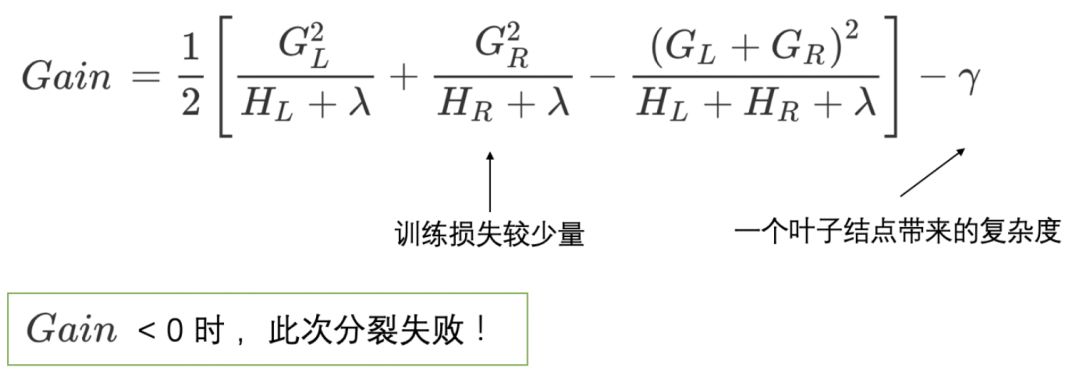
After splitting a new node, we need to check if this split brings a gain to the loss function, defined as:

If the gain Gain>0, meaning the objective function decreases after splitting into two leaf nodes, we will consider the results of this split.

However, when splitting a node, there may be many split points, and each split point will produce a gain. How can we find the optimal split point? This will be discussed next.

2. Finding the Best Split Point

When splitting a node, we will have many candidate split points. The general steps to find the best split point are as follows:

Iterate through each feature of each node;
For each feature, sort the feature values;
Linearly scan to find the best split feature value for each feature;
Find the best split point (feature and feature value with the largest gain) among all features

The above is a greedy method, where each split attempt requires a complete scan of all candidate split points, also known as the global scanning method.

However, when the data volume is too large, causing memory issues, or in distributed scenarios, the efficiency of the greedy algorithm becomes very low, and the global scanning method is no longer applicable.

Based on this, XGBoost has proposed a series of solutions to speed up the search for the best split point:

Feature Pre-sorting + Caching: XGBoost pre-sorts each feature by feature value before training, then saves it in a block structure. This structure will be reused in subsequent iterations, greatly reducing computation.
Quantile Approximation Method: After sorting each feature by feature value, it selects a constant number of feature values as candidate split points. When searching for the best split point for that feature, it selects the optimal one from the candidate split points.
Parallel Search: Since each feature is stored in a block structure, XGBoost supports using multiple threads to compute the best split point for each feature in parallel, which not only greatly enhances the speed of node splitting but also facilitates scalability for large training sets.

3. Stopping Growth

A tree will not grow indefinitely. Here are some common stopping criteria.

(1) When the gain from a new split is Gain<0, abandon the current split. This is a trade-off between training loss and model complexity.

(2) Stop growing the tree when it reaches its maximum depth, as a tree that is too deep is prone to overfitting. Here, a hyperparameter max_depth needs to be set.

(3) After a split, recalculate the sample weights for the newly generated left and right leaf nodes. If the sample weight of any leaf node falls below a certain threshold, that split will also be abandoned. This involves a hyperparameter: the minimum sample weight sum, which means that if a leaf node contains too few samples, the split will be abandoned to prevent the tree from becoming too fine, which is also a measure against overfitting.

The sample weight sum for each leaf node is calculated as follows:

Common Interview Questions

What are the advantages and disadvantages of XGB compared to GBDT and Random Forest?
Why can XGB train in parallel?
What are the advantages of using second-order Taylor expansion in XGB?
What designs has XGB implemented to prevent overfitting?
How does XGB handle missing values?
How does XGB split a node? How are features selected?
What conditions cause a tree in XGB to stop growing?
What do the weights of leaf nodes in XGB signify? How are they calculated?
What processes does training an XGB model involve? What are the parameter tuning steps?
How does XGB score features?

Interview Questions – Reference Answers:

Classic Interview Questions for XGBoost (Part 1)

Classic Interview Questions for XGBoost (Part 2)

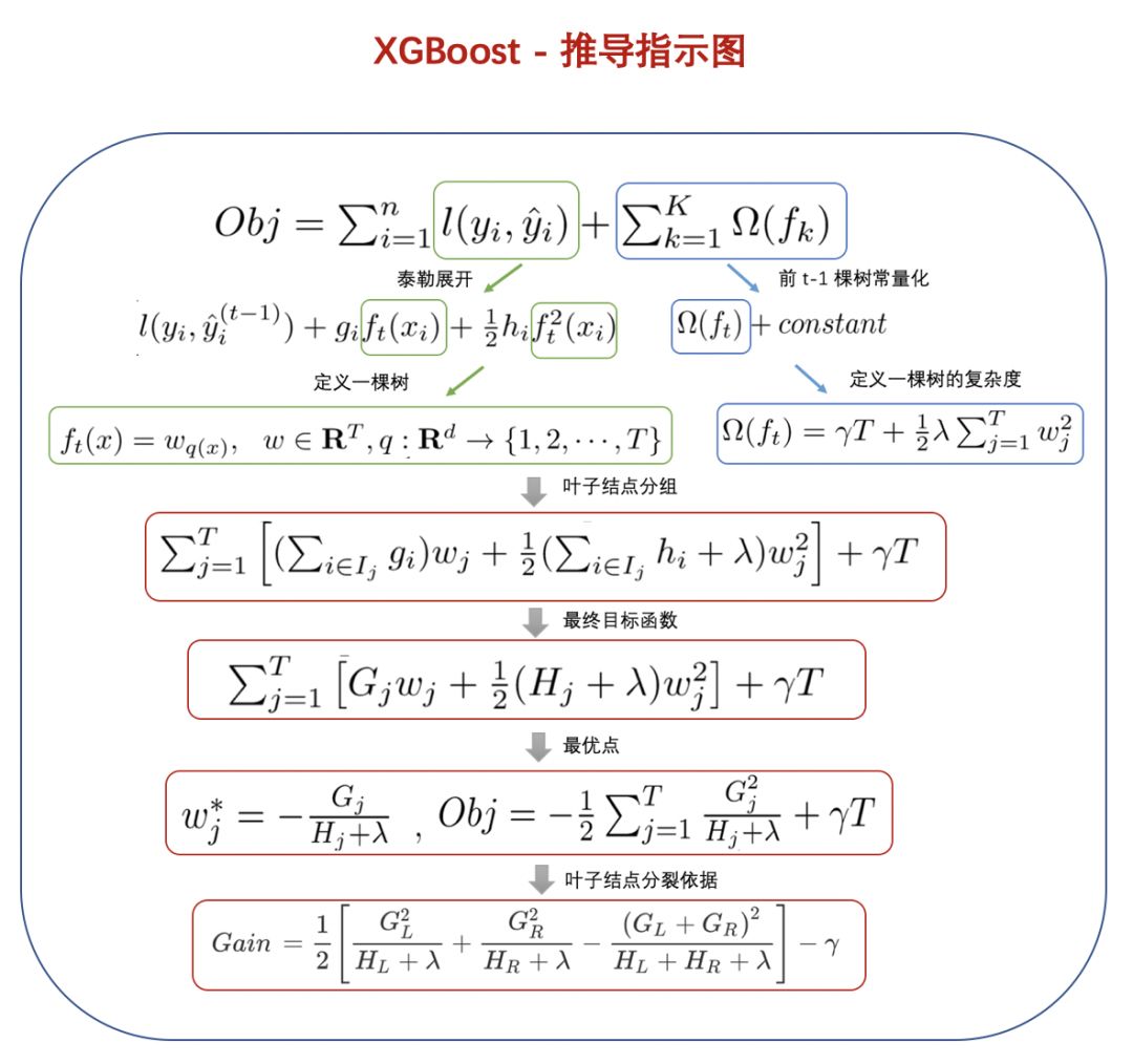
Cheat Sheet

After the detailed explanations in the previous sections, I believe everyone has a good understanding of the underlying principles of XGBoost. Below, I have prepared a cheat sheet to help everyone systematically grasp the entire derivation process of XGBoost principles while also serving as a quick reference.