Derivation of Backpropagation Algorithm in Convolutional Neural Networks (CNN)

First, I will introduce a simple method for analyzing the delta error backpropagation process. If the delta error of a certain node in layer l+1 needs to be transmitted to layer l, we look for which nodes in layer l are related to this node in layer l+1 during forward propagation and the weights involved. Then during backpropagation, the delta error will be multiplied by the same weight to propagate back.

Assume there is a node a in layer l and a node b in layer l+1. The connection weight between the two nodes is w. If during forward propagation, node a affects node b with a weight of . During backpropagation, the delta error of node b affects the delta error of node a. Their coefficients are the connection weights between the two nodes.

Brief Introduction to Forward Propagation Process in Convolutional Neural Networks

Before understanding the backpropagation of convolutional neural networks, we need to briefly review convolution, pooling, and the forward propagation process of convolutional neural networks.

Introduction to Convolution Operation

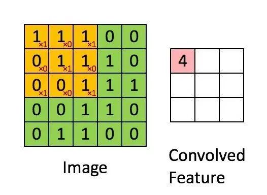
In convolutional neural networks, the so-called convolution operation is not strictly the convolution in the mathematical sense. The convolution in deep learning is actually the cross-correlation operation in signal processing and image processing, which has subtle differences. The convolution in deep learning (strictly speaking, cross-correlation) involves traversing the convolution kernel over the original image, multiplying corresponding elements and summing them up, resulting in a new image that is smaller in size. This can be intuitively understood through the following figure. Assuming the input image has m rows and n columns, and the size of the convolution kernel is filter_size × filter_size, the size of the output image will be (m-filter_size+1) × (n-filter_size+1).

In fully connected neural networks, image data and features are stored in the form of column vectors. In convolutional neural networks, the data format is mainly stored as tensors (which can be understood as multi-dimensional arrays). The format of the image is a three-dimensional tensor, rows × columns × channels. The format of the convolution kernel is a four-dimensional tensor, number of convolution kernels × rows × columns × channels.

The convolution operation takes out one convolution kernel at a time; a convolution kernel is three-dimensional, with rows × columns × channels. The image corresponding to the channel number undergoes a two-dimensional convolution operation with the convolution kernel (as shown in the above operation), resulting in the convolution result corresponding to that channel. The results of all channels are summed to obtain one channel of the output image. Each convolution kernel corresponds to one channel of the output image, meaning the number of channels in the output image equals the number of convolution kernels.

This concept may seem a bit convoluted, but the so-called tensor convolution in convolutional neural networks essentially involves a total of number of convolution kernels × number of channels two-dimensional convolution operations. Each convolution kernel corresponds to one channel of the convolution result, and each channel of the convolution kernel corresponds to one channel of the original image. This operation is somewhat analogous to multiplying a column vector by a matrix to obtain a new column vector.

The following figure intuitively demonstrates the specific operation process of tensor convolution:

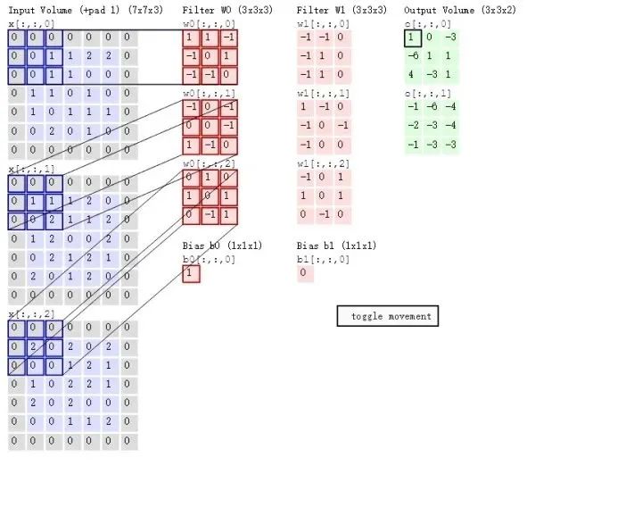
Introduction to Pooling Operation

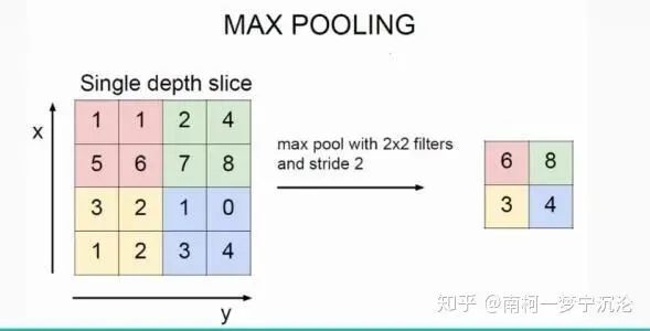
The so-called pooling refers to downsampling the image, where max pooling uses the maximum value of each region to represent that region, and average pooling uses the average value of each region to represent that region.

Derivation of Backpropagation in Convolutional Neural Networks

Backpropagation in Pooling Layer

The backpropagation in the pooling layer is relatively easy to understand. Taking max pooling as an example, in the image above, the number 6 after pooling corresponds to the red area before pooling. In fact, only the maximum value of 6 in the red area affects the pooled result, with a weight of 1, while the other numbers have no effect on the pooled result. Assuming the delta error at the position of the pooled number 6 is , when the error backpropagates, the delta error at the position corresponding to the maximum value in the red area will equal , while the delta errors at the other three positions will be 0.

Therefore, during forward propagation in max pooling of convolutional neural networks, it is necessary to not only record the maximum value of the region but also to record the position of the maximum value for the convenience of delta error backpropagation.

Average pooling is even simpler. Since in average pooling, each value in the region contributes equally to the pooled result, the delta error backpropagating will be the pooled delta error divided by the size of the region at each position.

Backpropagation in Convolutional Layer

Although the convolution operation in convolutional neural networks involves convolving a three-dimensional tensor image with a four-dimensional tensor convolution kernel, the core calculations only involve two-dimensional convolutions. Therefore, we will first analyze the two-dimensional convolution operation:

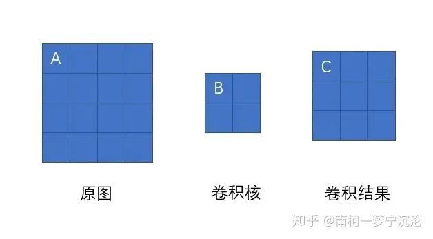
As shown in the figure above, to find the delta error at point A of the original image, we first analyze which nodes in the next layer it influences during forward propagation. Clearly, it only has an influence on node C with a weight of B, and has no influence on the other nodes in the convolution result. Therefore, the delta error at A should equal the delta error at point C multiplied by weight B.

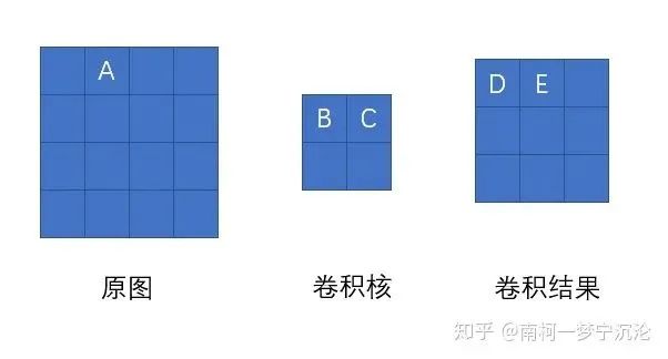
Now we will move the position of point A and see what the delta error at point A is after the transformation. Again, we first analyze which nodes in the convolution result it influences during forward propagation. After analysis, point A influences point D with weight C and point E with weight B. Thus, its delta error equals the delta error at point D multiplied by C plus the delta error at point E multiplied by B.

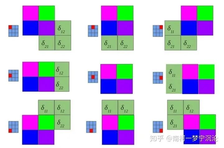
You can try to analyze the delta errors at other nodes in the original image using the same method. The result will show that the delta error of the original image equals the delta error of the convolution result after zero padding convolved with the convolution kernel rotated 180 degrees. As shown in the figure below:

Alright, we have an intuitive understanding. Next, we will prove this with mathematical formulas, even though they may be a bit tedious:

Let’s review the definition of delta error, which is the derivative of the loss function concerning the current layer’s unactivated output . We are now considering two-dimensional convolution, so the delta error at each layer is a two-dimensional matrix. It represents the delta error at coordinate (x, y) in layer l. Assuming we already know the delta error of layer l+1, we can easily write the following expression using the chain rule of differentiation:

Here, the coordinates (x’, y’) are the points in layer l+1 that are influenced by the coordinates (x, y) in layer l during forward propagation. There are multiple such points, and we need to sum them up. Then, using the relationship of forward propagation:

We can further expand the expression:

The long string at the end, although it looks complex, can actually be simplified quite easily:

At the same time, we obtain two constraints and :

Substituting the constraints into the above expression gives:

Then let and :

We have finally reached our conclusion:

We can celebrate briefly, but our current conclusion is still based on two-dimensional convolution. We still need to generalize it to the tensor convolution in our convolutional neural network.

Let’s review tensor convolution again. Each channel in the subsequent layer is obtained by convolving each channel of the previous layer and summing them up.

Wait, this relationship sounds a bit familiar. If we change channels to nodes and convolution to multiplication by weights, isn’t this somewhat similar to fully connected neural networks?

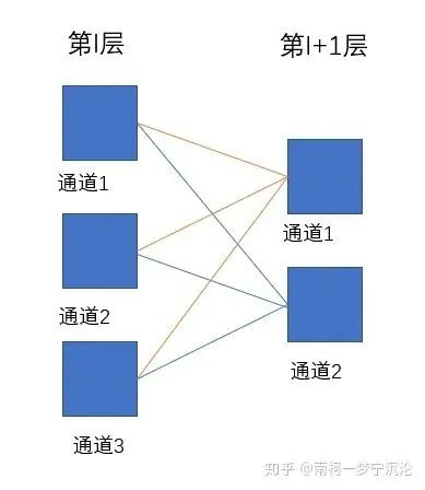
In the figure above, each line represents a convolution operation with a two-dimensional convolution kernel. Assuming the depth of layer l is 3 and the depth of layer l+1 is 2, the dimensions of the convolution kernel should be 2 × filter_size × filter_size × 3. The channel 1 of layer l influences the channels 1 and 2 of layer l+1 through convolution. Therefore, when calculating the delta error of channel 1 in layer l, we should simply sum the delta errors of channels 1 and 2 in layer l+1 according to the method of delta error propagation of the obtained two-dimensional convolution.

Given the delta error of layer l, calculate the derivative of the parameters of that layer

,

The convolution kernel in layer l is a four-dimensional tensor, with dimensions representing the number of convolution kernels × number of rows × number of columns × number of channels. In practice, it can be viewed as having convolution kernels × number of channels two-dimensional convolution kernels, each corresponding to the corresponding channels of the input image and output image. Each two-dimensional convolution kernel only involves one two-dimensional convolution operation. Therefore, to obtain the derivative of the entire convolution kernel, we only need to analyze the derivatives of each two-dimensional convolution kernel in the convolution of convolution kernels × number of channels and then combine them into a four-dimensional tensor.

Thus, we analyze the two-dimensional convolution:

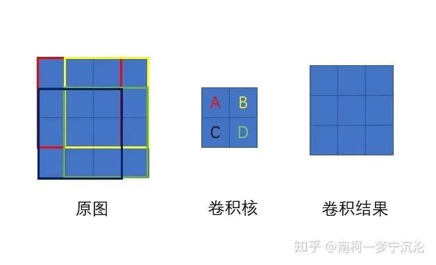
Using the previous analysis method, point A on the convolution kernel clearly affects every point of the convolution result. Its influence on the convolution result equals multiplying the entire upper left 3×3 part of the original image by the value at point A. Therefore, when the delta error backpropagates, the derivative at point A equals the convolution result’s delta error summed with the original image’s upper left 3×3 red section. Thus, the derivative of the two-dimensional convolution kernel equals the convolution of the delta error corresponding to the output image’s channel with the original image’s corresponding channel.

We will then recombine the derivatives of the number of original image channels × number of convolution result channels two-dimensional convolution kernels into a four-dimensional tensor to obtain the derivative of the entire convolution kernel.

Next, we will derive from mathematical formulas:

Similarly, we can simplify and obtain two constraints: and :

This time, we do not need to perform the 180-degree rotation operation.

Given the delta error of layer l, calculate the derivative of the parameters of that layer

Our is a column vector, which adds the same scalar to each channel of the convolution result. Therefore, during backpropagation, its derivative equals the sum of the convolution result’s delta error across each channel.

Here is a simple formula proof:

Since is 1

Thus:

Proved

Convolutional neural networks include convolution layers, pooling layers, and fully connected layers. This article introduces the backpropagation algorithm for convolution and pooling layers and the calculation method for the parameters’ derivatives at each layer. The backpropagation method for fully connected layers and the calculation of parameter derivatives have also been introduced in previous articles.

Let us summarize the training process of convolutional neural networks:

1. Initialize the neural network, define the network structure, set the activation function, randomly initialize the convolution kernel W and bias b for the convolution layer, and randomly initialize the weight matrix W and bias b for the fully connected layer. Set the maximum number of iterations for training, the batch size for each training batch, and the learning rate.
2. Take a batch of data from the training data.
3. From that batch of data, take one data point, including input x and the corresponding correct label y.
4. Feed input x into the input end of the neural network to obtain the output parameters of each layer of the neural network.
5. Calculate the loss function of the neural network based on the output and the label value y.
6. Calculate the delta error of the loss function concerning the output layer.
7. Use the recursive formula for delta errors between adjacent layers to find the delta error for each layer, if it is a fully connected layer, if it is a convolution layer, if it is a pooling layer.
8. Use the delta error for each layer to calculate the derivative of the loss function concerning the parameters of that layer, if it is a fully connected layer, if it is a convolution layer.
9. Add the derivatives obtained from the current batch of data to the sum of derivatives initialized to 0, jump back to step 3 until all data in the batch is trained.
10. Use the sum of derivatives obtained from one batch of data to update the parameters according to the gradient descent method.
11. Jump back to step 2 until the specified number of iterations is reached.

References: