Excerpt from THE ASIMOV INSTITUTE
Author: FJODOR VAN VEEN
Translation by Machine Heart
Contributors: Huang Xiaotian, Li Yazhou
In September 2016, Fjodor Van Veen wrote an article titled “The Neural Network Zoo” (see the illustrated overview of neural network architectures: from basic principles to derivatives), which comprehensively reviewed a multitude of frameworks for neural networks and illustrated them with intuitive diagrams. Recently, he published a follow-up article titled “The Neural Network Zoo Prequel: Cells and Layers,” which serves as a prelude to his previous work, providing a richly illustrated introduction to the units and layers of neural networks that were mentioned but not elaborated upon in the original article. Machine Heart has translated this article, with the original link provided at the end.

Cell
The article “The Neural Network Zoo” showcased different types of units and various layer connection styles, but did not delve into how each unit type operates. A variety of unit types possess different colors to clearly differentiate networks, yet I have found that these units function quite similarly. Below, I describe each unit in detail.
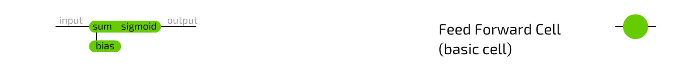
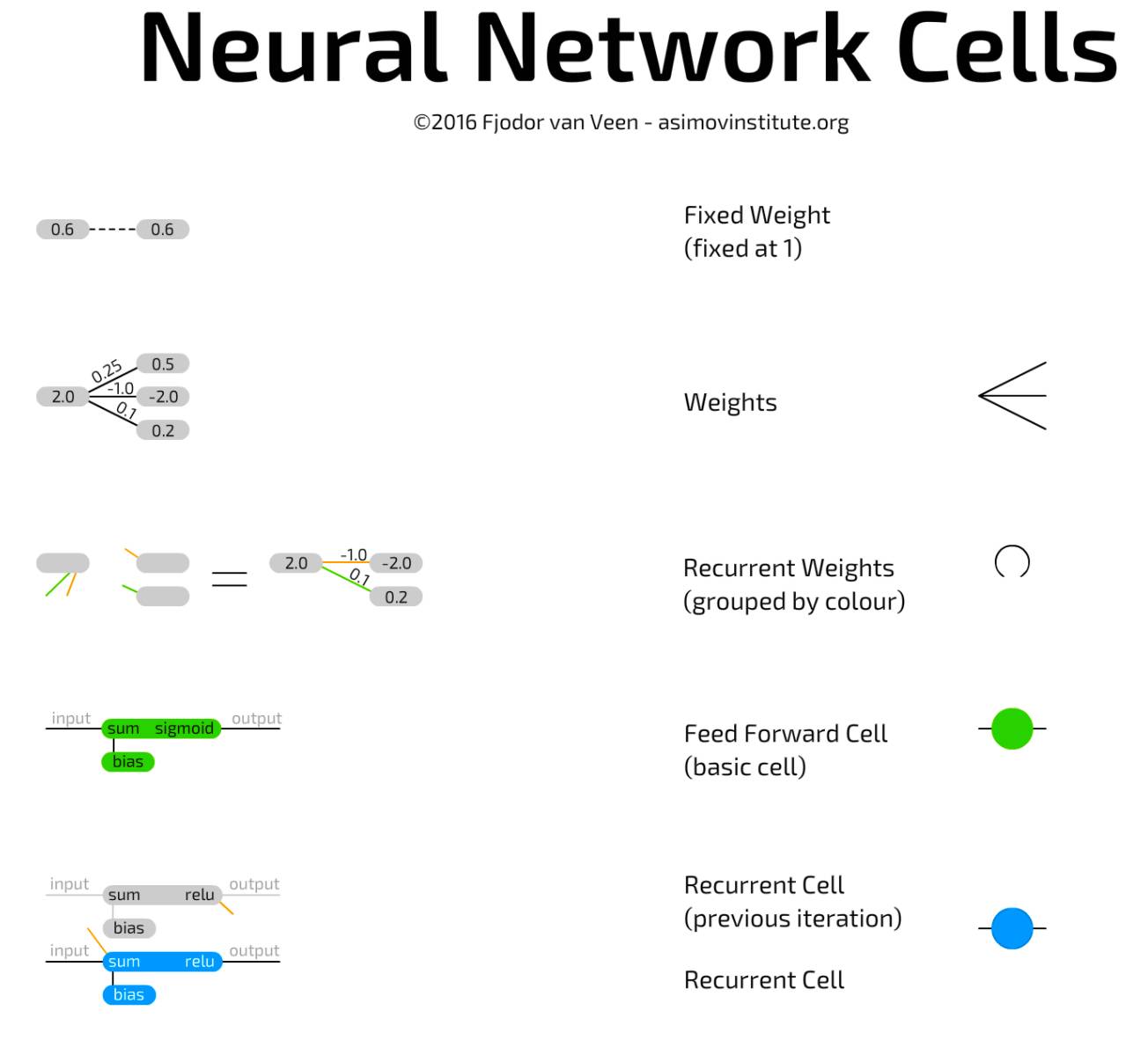
Basic Neural Network Unit is a type belonging to conventional feedforward architectures and is quite simple. The unit connects to other neurons through weights, meaning it can connect to all neurons in the previous layer. Each connection has its own weight, which is often a random number at the start. A weight can be negative, positive, small, large, or zero. Each unit value it connects to is multiplied by its respective connection weight, and the resulting values are summed up. Additionally, a bias term is added at the top. The bias term can prevent the unit from outputting zero, speeding up its operation, and reducing the number of neurons required to solve a problem. The bias term is also a number, sometimes a constant (usually -1 or 1), and sometimes a variable. This total is then passed to the activation function, and the resulting value is the unit value.
Convolutional Unit is similar to the feedforward unit, except that the former typically connects to only a few neurons in the previous layer. They are commonly used to preserve spatial information, as they connect not to a few random units, but to all units within a certain distance. This makes them well-suited for processing data with a lot of local information, such as images and audio (mostly images). The deconvolutional unit works in opposition to the convolutional unit: it tends to decode spatial information by connecting locally to the next layer. The two units usually have independently trained clones, each with its weights, and connected in the same manner. These clones can be seen as separate networks with the same structure. Both are essentially the same as conventional units but used differently.
Pooling and Interpolating Units frequently connect with convolutional units. These units are not actually units, but rather primitive operations. The pooling unit receives input connections and decides which connections are allowed to pass through. In images, this can be seen as reducing the size of the picture. You no longer see all the pixels, and it has to learn which pixels to keep and which to discard. The interpolating unit performs the opposite operation; it receives some information and maps it to more information. The additional information is composed, like enlarging a low-resolution image. The interpolating unit is not the only reverse operation of the pooling unit, but the two are relatively common due to their quick and simple implementation. They connect in a manner similar to convolution and deconvolution.
Mean and Standard Deviation Units (almost entirely found as probabilistic units in pairs) are used to characterize probability distributions. The mean is simply the average, while the standard deviation indicates how far it can deviate from this mean in both directions. For example, a probability cell for an image might contain information about how much red is present in a specific pixel. For instance, a mean of 0.5 and a standard deviation of 0.2. When sampling from these probability units, these values need to be input into a Gaussian random number generator, where values between 0.4 and 0.6 are likely outcomes; those far from 0.5 are less likely (but still possible). Mean and standard deviation cells are often fully connected to the previous or next layer, and do not have a bias.
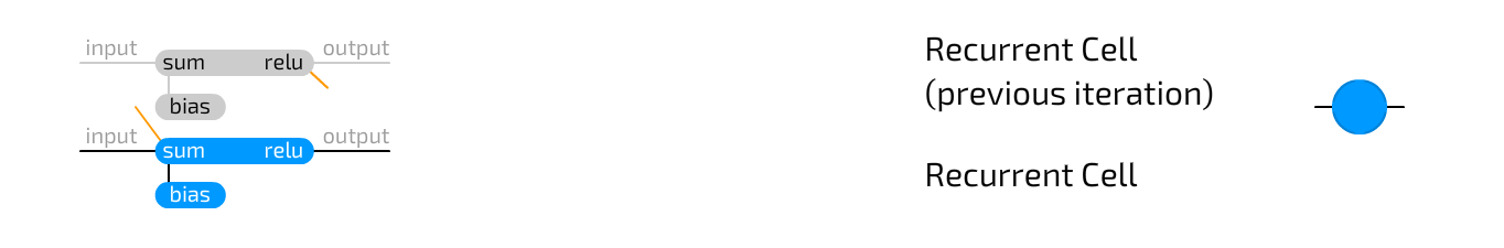
Recurrent Unit connects not only to layers but also has connections over time. Each unit internally stores previous values. They are updated like basic units, but with additional weights: connections to previous values of the unit, and most of the time also connecting to all units in the same layer. These weights between the current value and the stored previous value function more like volatile memory, similar to RAM, which retains a specific “state” attribute, but disappears if not fed. Since previous values are passed to the activation function, and the activated value is passed along with other weights through each update, information will continually be lost. In fact, the retention rate is so low that after 4 to 5 iterations, almost all information is lost.
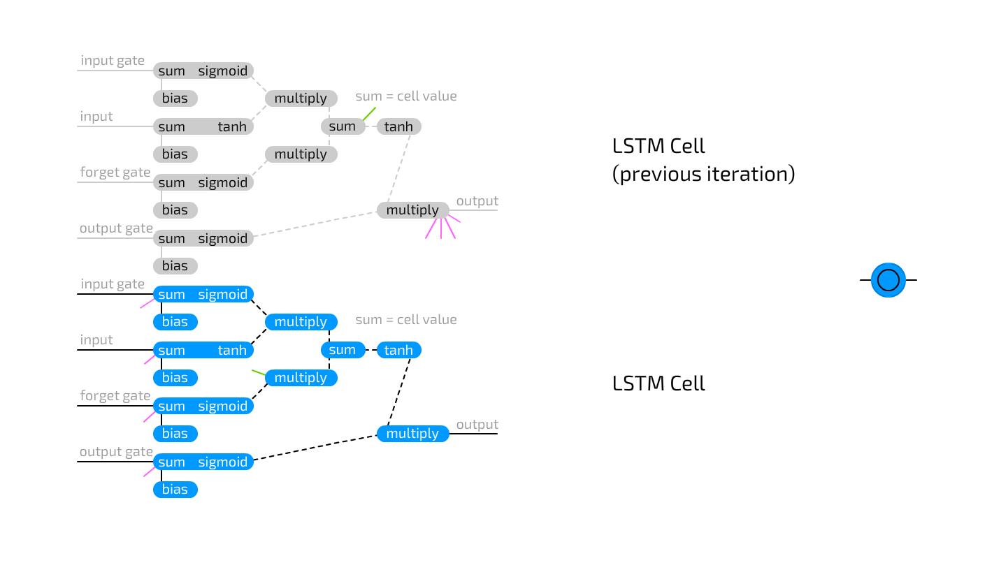
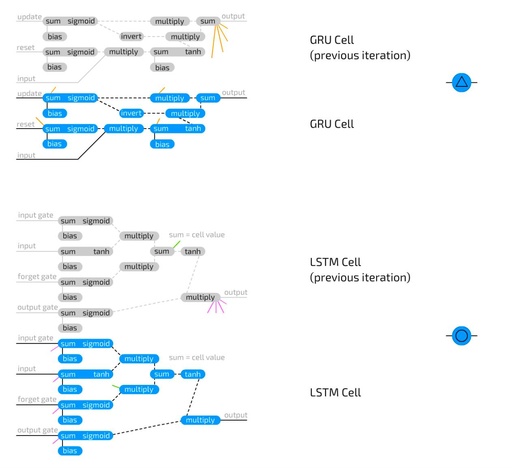
Long Short-Term Memory Unit is used to address the rapid information loss occurring in recurrent units. LSTM units are logical circuits that replicate the way memory units are designed for computers. Compared to RNN units that store two states, LSTM units can store four: the current output value and final value, as well as the current and final values of the “memory unit” state. LSTM units contain three “gates”: input gate, output gate, and forget gate, and also include conventional inputs. Each of these gates has its own weights, meaning that connections to this type of cell require setting four weights (instead of just one). The gate functions are like flow gates, rather than fence gates: they can let anything through, just a little, none, or anything in between. This operates by multiplying the input information stored in this gate value, which ranges from 0 to 1. The input gate then decides how much input can be added to the unit value. The output gate determines how many output values can be seen by the remaining network. The forget gate does not connect to the previous value of the output unit but connects to the previous memory unit value. It decides how much of the final memory unit state to retain. Since it does not connect to the output, less information is lost, as no activation function is placed in the cycle.
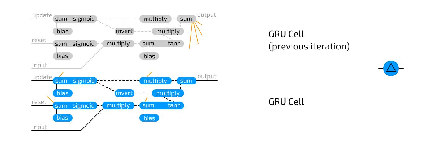
Gated Recurrent Unit is a variant of LSTM. They also use gates to prevent information loss but only have two gates: update gate and reset gate. This is slightly less expressive but faster, as they have fewer connections everywhere. In fact, there are two differences between LSTM and GRU: GRU does not protect the hidden unit state with an output gate but combines the input and forget gates into one update gate. The idea is that if you want a lot of new information, you can forget some old information (or vice versa).
Layers
The most basic way to connect neurons into a graph is to interconnect everything, which can be seen in Hopfield networks and Boltzmann machines. Of course, this means the number of connections grows exponentially, but the expressiveness is undeniable. This is known as fully connected.
Subsequently, it was discovered that it is useful to divide the network into different layers, where a series or group of neurons in one layer do not connect to each other but connect to neurons in other groups. For example, in the restricted Boltzmann machine’s network layers. Today, the concept of layers has been extended to any number of layers and can be seen in almost all architectures. This is also referred to as fully connected (which can be a bit confusing), as fully connected networks are actually quite rare.
Convolutional Connection Layer is more restricted than a fully connected layer: each neuron only connects to nearby neurons in other groups. Images and audio contain a lot of information that cannot be used one-to-one for direct feeding into the network (e.g., one neuron corresponds to one pixel). The idea of convolutional connections comes from the observation of preserving important spatial information. It turns out to be a good idea, used in many image and speech applications based on neural networks. However, this setup is less expressive than fully connected layers. In fact, it is a way of filtering for “importance,” deciding which are important among these compact data packets. Convolutional connections are also great for dimensionality reduction. Thanks to its implementation, even neurons that are spatially far apart can connect, but neurons with a range higher than 4 or 5 are rarely used. Note that here, “space” typically refers to two-dimensional space, using this two-dimensional space to express the three-dimensional surface of neuron connections. The range of connections can be applied in all dimensions.
Another option is of course randomly connected neurons. It has two main variants: allowing a portion of all possible connections or connecting a portion of neurons between layers. Random connections help linearly reduce network performance and can be used for fully connected layers in large networks that are prone to performance issues. In some cases, a sparser connection layer with more neurons performs better, especially when there is a lot of information to store but not exchange (somewhat similar to the effectiveness of convolutional connection layers, but random). As seen in ELM, ESN, and LSM, very sparse connection systems (1% or 2%) are also used. Particularly in spiking networks, because the more connections a neuron has, the less energy each weight carries, meaning less propagation and pattern repetition.
Delayed Connections refer to neurons not obtaining information from the previous layer but from the past (mostly from previous iterations). This allows temporal information (time, sequence) to be stored. These connections sometimes need to be manually reset to clear the network’s “state.” The main difference from conventional connections is that these connections continuously change, even when the network is not being trained.
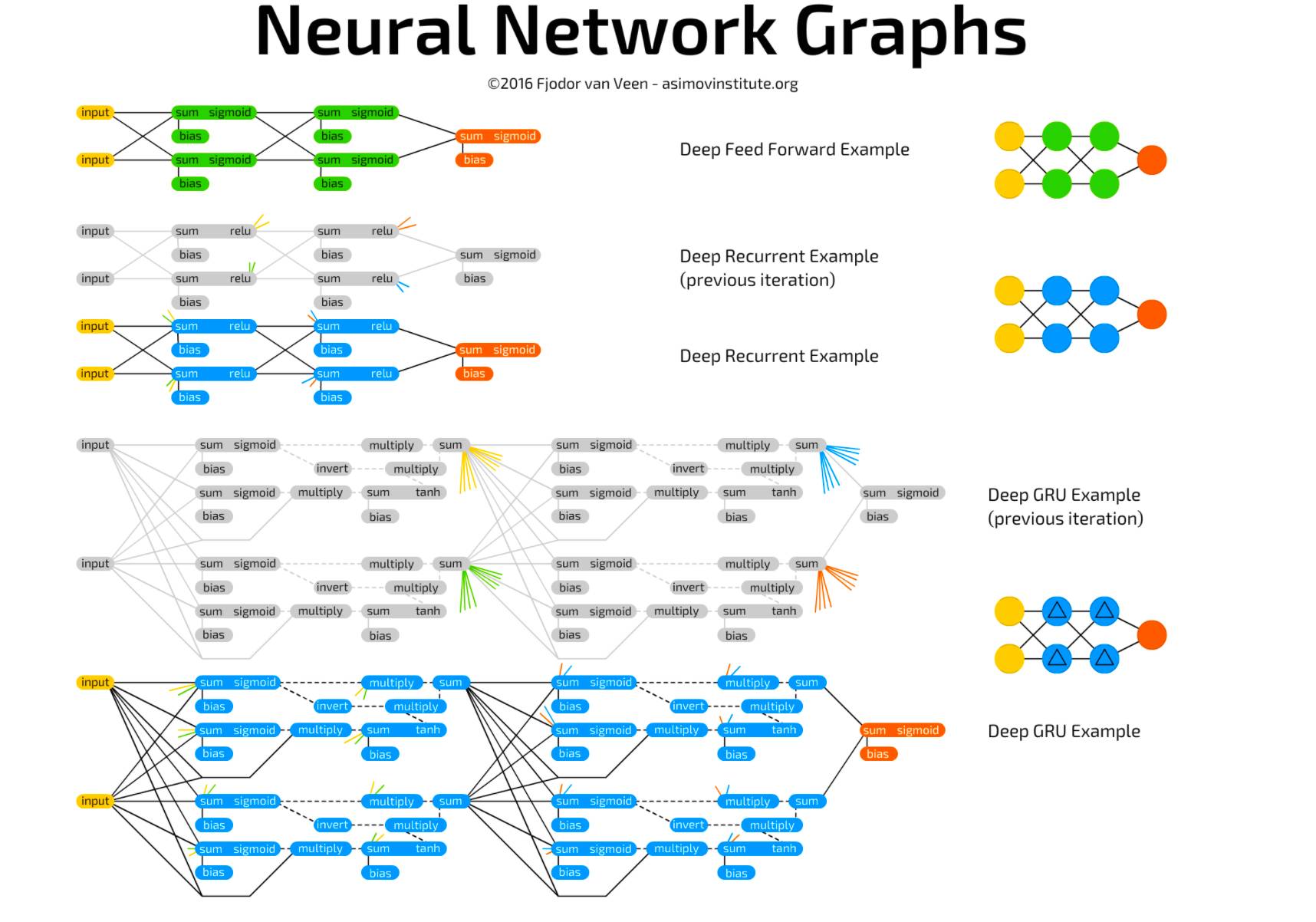
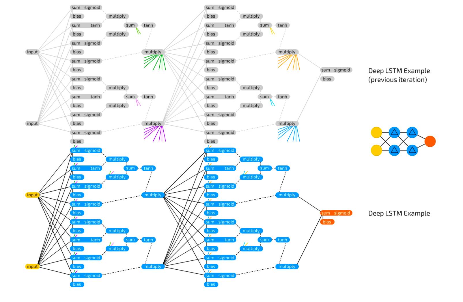
The following images show some small sample networks and their connections based on the descriptions above. When I am unsure what connects to what, I will use this (especially when making LSTM or GRU cells):
Original link: http://www.asimovinstitute.org/neural-network-zoo-prequel-cells-layers/
This article is a translation by Machine Heart, please contact this public account for authorization to reprint.
✄————————————————
Join Machine Heart (Full-time Journalist/Intern): [email protected]
Submissions or Reporting Inquiries: [email protected]
Advertising & Business Cooperation: [email protected]
Click to read the original text, visit the Machine Heart official website↓↓↓