One-Shot Learning with Deep Neural Networks: Siamese Networks for Few-Shot Classification

1New Intelligence Compilation

Source: sorenbouma.github.io

Author: Soren Bouma

Compilation: Jiang Hongliang

[New Intelligence Guide]This blog is translated from One Shot Learning and Siamese Networks in Keras. This article will introduce One-shot Learning, describe the benchmark for single-sample classification problems, combine an example (including implementation code), and point out some small ideas that people usually do not think of. Study hard!

Background

Traditionally, it is generally believed that deep neural networks are good at learning from high-dimensional data, such as images or language, but this is based on the condition that they have a large number of labeled samples for training. However, humans possess the ability of one-shot learning—if you show a person who has never seen a small shovel a picture of it, they should be able to efficiently distinguish it from other kitchen utensils.

This is a task that is easy for humans, but when we want to write an algorithm to do it… that’s when it gets tricky. It is clear that machine learning systems would love to have this ability to quickly learn from a small number of samples, as collecting and labeling data is a time-consuming and labor-intensive task. Moreover, I believe this is an important step on the long road to general artificial intelligence.

Recently, many interesting one-shot learning papers based on neural networks have emerged, achieving some good results. This is an exciting new field for me, so I want to give a brief introduction to help newcomers in deep learning better understand it.

In this blog, I want to:

• Introduce and define the one-shot learning problem

• Describe the benchmark for one-shot classification problems and provide a baseline for its performance

• Provide an example of few-shot learning and partially implement the model mentioned in this paper

• Point out some small ideas that people usually do not think of

Defining the Problem: N-Class One-Shot Learning

Before we solve any problem, we should precisely define what the problem is. Below is the symbolic representation of the one-shot classification problem: Our model has only a few labeled training samples S, which has N samples, each a vector of the same dimension.Each has a corresponding label y.

Then we have a test sample to classify . Because each sample in the sample set has a correct category , our goal is to correctly predict which one is the correct label in y∈S.

There are many ways to define the problem, but the above is our definition. Note that there are some things to record here:

• In real life, there may be fewer constraints; one image may not necessarily have only one correct category

• This problem can easily generalize to k-shot learning, we just need to replace each category with k samples

• When N is high, there may be more possible categories, making correct category prediction more difficult

• The correct rate for random guessing is

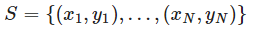
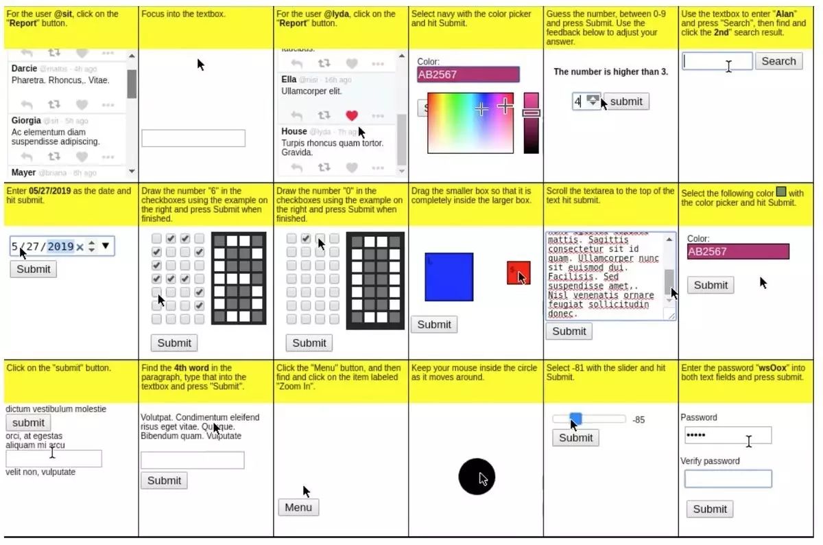
Here are some examples of one-shot learning on the Omniglot dataset, which I will introduce in the next section. The illustrations represent one-shot learning tasks of 9 classes, 25 classes, and 36 classes.

About the Omniglot Dataset!

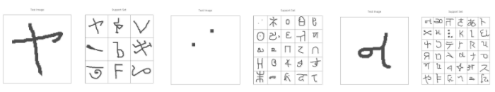
The Omniglot dataset contains 50 scripts and 1623 classes of handwritten characters. For each class of characters, there are only 20 samples, each drawn by different people, with a resolution of 105*105.

Above are some examples from the Omniglot dataset. As shown in the figure, there are many characters. If you like machine learning, you must have heard of the MNIST dataset. Omniglot is sometimes referred to as the transposed MNIST because it has 1623 classes of characters, with only 20 samples per class, in contrast to MNIST’s 10 classes, each with thousands of samples. Omniglot also has stroke data, but we won’t use it here.

Typically, we divide the samples into 30 classes for training and the remaining 20 classes for evaluation. All these different characters can compose many one-shot learning tasks, so it is indeed a good benchmark for one-shot learning.

A One-Shot Learning Baseline: 1-Nearest Neighbor

The simplest classification method is to use the k-nearest neighbors method, but since each category has only one sample, we need to use 1-nearest neighbor. This is simple; we just need to calculate the Euclidean distance between the test sample and each sample in the training set and then select the nearest one:

According to Koch et al.’s paper, on 20 classes in the Omniglot dataset, one-shot classification with 1-nn can achieve about 28% accuracy. 28% seems poor, but it is already 6 times better than random guessing (5%). This is the best baseline or “sanity check” for one-shot learning algorithms.

Lake et al.’s Hierarchical Bayesian Program Learning (HBPL) achieved about 95.2% accuracy, which is impressive. I only understood 30% of it, but it is very interesting. It is completely different from deep learning, which trains directly from raw pixels, because:

1. HBPL uses stroke data rather than just raw pixels;

2. HBPL learns a generative model of strokes on the Omniglot dataset, which requires more complex annotations, unlike deep learning that can directly do one-shot learning from raw pixels of images of dogs, trucks, brain scans, and small shovels, which are not composed of strokes.

Lake et al. also pointed out that humans can achieve 95.5% accuracy on the 20-class samples of the Omniglot dataset, just slightly higher than HBPL. Guided by the idea of drilling down, I personally experimented with the 20-class task, achieving 97.2% accuracy. I was not doing true one-shot learning because there were many symbols I already recognized; I removed those I was familiar with, such as Greek letters, hiragana, and katakana, and still achieved 96.7% accuracy. I think it is because I have developed superhuman character recognition abilities from my own terrifying handwriting.

Using Deep Neural Networks for One-Shot Learning?!

If we simply train a softmax classifier neural network with cross-entropy loss for one-shot learning, it is clear that the network will severely overfit. Even if given hundreds of samples per category, modern neural networks still overfit. Deep networks have millions of parameters to fit training data, so they can learn a huge function space (formally, this is because they have a high VC dimension, which is part of why they can learn well from complex high-dimensional data).

Unfortunately, this advantage of neural networks becomes a major obstacle for them to perform one-shot learning. When there are millions of parameters needing gradient descent, with so many possible mappings to learn, how can we design a network to learn from a single sample?

Humans easily learn the meaning of a small shovel or the letter Θ from a single sample because we have spent a lifetime observing and learning from similar objects. It is indeed unfair to compare a randomly initialized neural network with humans who have spent a lifetime recognizing objects and symbols because the randomly initialized neural network lacks prior knowledge of the data’s mapping structure. This is also why I see that one-shot learning papers all adopt knowledge transfer methods from other tasks.

Neural networks are very good at extracting features from structured complex/high-dimensional data (like images). If given training data similar to the one-shot learning task, they might be able to learn useful features from this data that can be applied to one-shot learning without adjustment. Thus, we can still call it one-shot learning because the auxiliary training data and the one-shot test data are not of the same category.(Note: The features here refer to “the mapped data of the training data”—translator’s note: for example, features extracted by CNN).

Next, an interesting question is how do we design a neural network for it to learn features? The most obvious way is to use transfer learning (if labeled data is available)—train a softmax classifier on the training data and then fine-tune the weights of the last layer on the one-shot learning task dataset. In fact, neural network classifiers do not perform well on the Omniglot dataset because each category has only a few samples, and even fine-tuning the weights of the last layer, the network will overfit on the training set. But this method is still much better than using the L2 distance k-nearest neighbor method (refer to Matching Networks for One Shot Learning for a comparison of various one-shot learning methods’ effectiveness).

There is still a way to do one-shot learning! Forget the 1-nearest neighbor method? This simple, non-parametric one-shot learner calculates the L2 distance between samples in the test set and each sample in the training set and selects the nearest one as its category. This method is okay, but L2 distance suffers from severe dimensionality disaster problems, so it does not perform well on high-dimensional data (like Omniglot).

Additionally, if you have two nearly identical images, if you slightly shift the pixels of one image to the right, the L2 distance between the two images will suddenly increase from 0 to very high. L2 distance is a terrible metric for such tasks. Can deep learning work? We can use deep convolutional neural networks to learn a similarity function that can be used by a non-parametric nearest neighbor classifier.

Siamese Networks

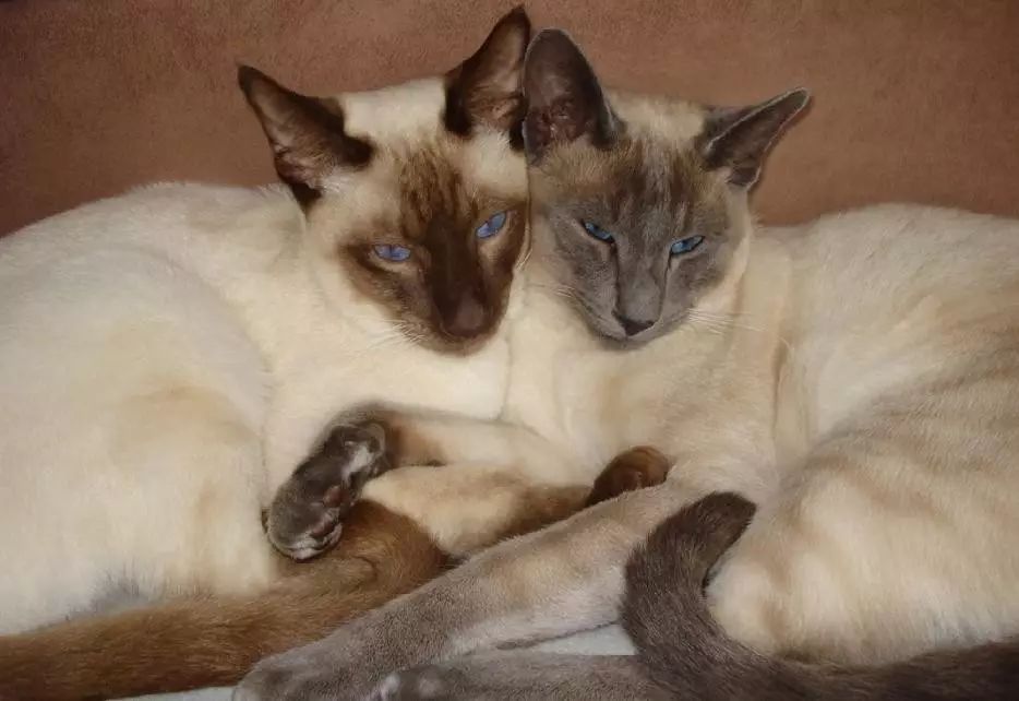
I originally intended to put a picture of conjoined twins as an introductory image for this section, but I ultimately thought an image of Siamese kittens might be better.

In this tutorial, I will implement a method from an excellent paper (Siamese Neural Networks for One-shot Image Recognition). The one-shot learning method by Koch et al. simultaneously gives the neural network two images to guess whether the two images belong to the same category. When we perform the one-shot classification task mentioned above, the network can compare each image in the test set with each image in the training set and select which one is most likely to be the same category. Therefore, we want the neural network architecture to take two images as input and output the probability that they belong to the same category.

Assume and are two categories in the dataset. We let represent that and are the same category. Note that and are equivalent—this means that if we reverse the order of the input images, the output probabilities will be the same.This is called symmetry, and Siamese networks are designed based on it.

Symmetry is very important because it learns a distance metric— to ‘s distance should equal to to ‘s distance.

If we simply concatenate the two samples and treat it as a single input to the neural network, each sample will be multiplied by a matrix with a different set of weights (or entangled), which will break the symmetry. No problem, such a network can still successfully learn the same weights for each input, but it is easier to learn the same weights for both inputs. Therefore, we can let both inputs pass through exactly the same network with shared parameters, and then use the absolute difference as input to a linear classifier—this is the necessary structure of the Siamese network. Two identical twins sharing a head, that’s where the name Siamese Network comes from.

CNN Siamese Network Architecture

Unfortunately, if we want to clearly introduce why convolutional neural networks can work, this blog will become long. If you want to understand convolutional neural networks, I suggest you study CS231 and then go to Colah. For readers without deep learning experience, I can only summarize CNN like this:

An image is a 3D pixel matrix, a convolutional layer is a neuron connected to a small part of the previous layer of neurons (translator’s note: local connectivity, e.g., using a 3*3 convolution kernel), and then sliding over an image or feature block with the same connection weights to generate another 3D neuron. A max pooling layer is used to spatially reduce the feature map. Stacking many such layers in sequence can be trained using gradient descent, and they perform well on image tasks.

I only give a brief introduction to CNN because this is not the focus of this article. Koch et al. used convolutional Siamese networks to classify paired Omniglot images, so both Siamese networks are convolutional neural networks. The architecture of each of these two Siamese networks is as follows: 64 channels with a 10×10 convolution kernel, relu->max pool->128 channels with a 7×7 convolution kernel, relu->max pool->128 channels with a 4×4 convolution kernel, relu->max pool->256 channels with a 4×4 convolution kernel.

The Siamese network reduces the input to smaller and smaller 3D tensors, and finally passes through a fully connected layer with 4096 neurons. The absolute difference between the two vectors is used as input to the linear classifier. This network has a total of 38,951,745 parameters—96% of the parameters belong to the fully connected layer. This amount of parameters is large, so the network has a high risk of overfitting, but the paired training means the dataset is large, so the overfitting problem does not occur.

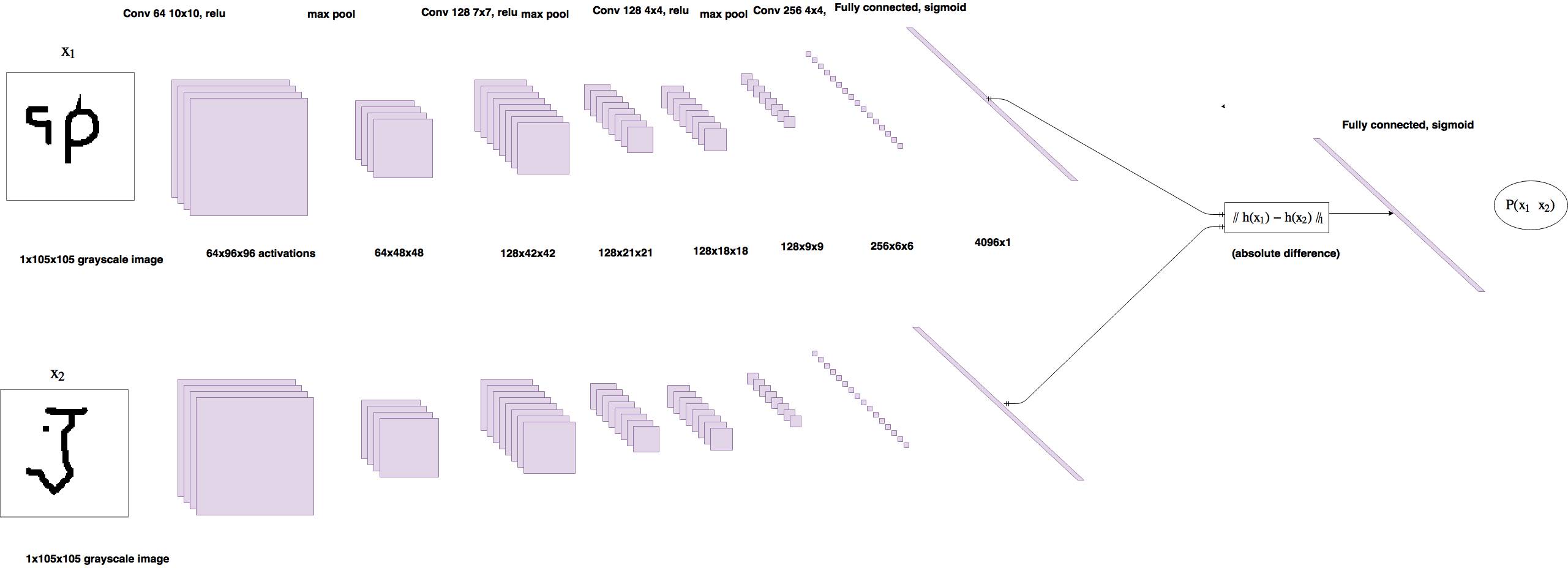
Sketch of the architecture

The output is normalized to [0,1] using the sigmoid function to make it a probability. When the two images are of the same category, we set the target t=1, and when they are of different categories, we set t=0. It uses logistic regression for training. This means the loss function should be the binary cross-entropy between the prediction and the target. The loss function also includes an L2 weight decay term to allow the network to learn smaller or smoother weights, thus improving generalization:

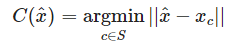
When the network performs one-shot learning, the Siamese network simply classifies which test image is most similar to the images in the training set:

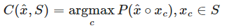
Here we use argmax instead of argmin in the nearest neighbor method because the more different the categories, the higher the L2 metric value, but the output of this model is , so we want this value to be maximized. This method has a clear drawback: for any in the training set, the probabilities are independent of each sample in the training set! This means the sum of probability values is not equal to 1. In any case, the test image and training image should be of the same type…

Observation: Size of Effective Dataset for Paired Training

After discussions with PhD students at UoA, I found that this is exaggerated or just wrong. Empirically, my implementation did not overfit, even if it did not train sufficiently on every possible paired image, which conflicts with this section. Guided by the idea of correcting mistakes, I will keep this question open. (This is probably the original author’s self-talk~)

I noticed that using paired training would result in a quadratic number of image pairs to train the model, which makes it hard for the model to overfit, which is cool. Suppose we have E classes, each with C samples. There are a total of C⋅E images, and the total possible pairing can be calculated as follows:

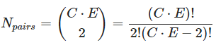
For the 964 classes in Omniglot (20 samples per class), this results in 185,849,560 possible pairs, which is huge! However, Siamese networks need both same-class and different-class pairs. Each class has E training samples, so each category has same-category pairs. This means there are 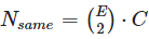same-category pairs for Omniglot. Even 183,160 pairs is large, but it is only one-thousandth of all possible pairs because the number of same-category pairs increases quadratically with E, while C increases linearly. This issue is very important because when training Siamese networks, the ratio of same-category to different-category pairs should be 1:1. Perhaps it indicates that paired training is easier to train on datasets with more samples per category.

Code

If you prefer using Jupyter Notebook, here is the link: https://github.com/sorenbouma/keras-oneshot

Below is the model definition. If you are familiar with Keras, it will be easy to understand. I only use Sequential() to define the Siamese network once, then call it using two input layers so that both inputs use the same parameters. Then we merge them using absolute distance and add an output layer, compiling this model using binary cross-entropy loss.

from keras.layers import Input, Conv2D, Lambda, merge, Dense, Flatten, MaxPooling2D
from keras.models import Model, Sequential
from keras.regularizers import l2
from keras import backend as K
from keras.optimizers import SGD, Adam
from keras.losses import binary_crossentropy
import numpy.random as rng
import numpy as np
import os
import dill as pickle
import matplotlib.pyplot as plt
from sklearn.utils import shuffle

def W_init(shape,name=None):
    """Initialize weights as in paper"""
    values = rng.normal(loc=0,scale=1e-2,size=shape)
    return K.variable(values,name=name)#//TODO: figure out how to initialize layer biases in keras.

def b_init(shape,name=None):
    """Initialize bias as in paper"""
    values=rng.normal(loc=0.5,scale=1e-2,size=shape)
    return K.variable(values,name=name)

input_shape = (105, 105, 1)
left_input = Input(input_shape)
right_input = Input(input_shape)
#build convnet to use in each siamese 'leg'
convnet = Sequential()
convnet.add(Conv2D(64,(10,10),activation='relu',input_shape=input_shape,
                   kernel_initializer=W_init,kernel_regularizer=l2(2e-4)))
convnet.add(MaxPooling2D())
convnet.add(Conv2D(128,(7,7),activation='relu',
                   kernel_regularizer=l2(2e-4),kernel_initializer=W_init,bias_initializer=b_init))
convnet.add(MaxPooling2D())
convnet.add(Conv2D(128,(4,4),activation='relu',kernel_initializer=W_init,kernel_regularizer=l2(2e-4),bias_initializer=b_init))
convnet.add(MaxPooling2D())
convnet.add(Conv2D(256,(4,4),activation='relu',kernel_initializer=W_init,kernel_regularizer=l2(2e-4),bias_initializer=b_init))
convnet.add(Flatten())
convnet.add(Dense(4096,activation="sigmoid",kernel_regularizer=l2(1e-3),kernel_initializer=W_init,bias_initializer=b_init))
#encode each of the two inputs into a vector with the convnet
encoded_l = convnet(left_input)
encoded_r = convnet(right_input)
#merge two encoded inputs with the l1 distance between them
L1_distance = lambda x: K.abs(x[0]-x[1])
both = merge([encoded_l,encoded_r], mode = L1_distance, output_shape=lambda x: x[0])
prediction = Dense(1,activation='sigmoid',bias_initializer=b_init)(both)
siamese_net = Model(input=[left_input,right_input],output=prediction)
#optimizer = SGD(0.0004,momentum=0.6,nesterov=True,decay=0.0003)

optimizer = Adam(0.00006)
#//TODO: get layerwise learning rates and momentum annealing scheme described in paperworking

siamese_net.compile(loss="binary_crossentropy",optimizer=optimizer)

siamese_net.count_params()

In the original paper, each layer has different learning rates and momentum—I skipped this step because it is too cumbersome to implement this in Keras, and hyperparameters are not the focus of this paper. Koch et al. added distorted images to the training set, using 150,000 pairs of samples to train the model. Because this is too large, my memory cannot hold it, so I decided to use random sampling. Loading image pairs may be the most difficult part of implementing this model. Since each class has 20 samples, I reshaped the data into an N_classes×20×105×105 array for easy indexing.

class Siamese_Loader:
    """For loading batches and testing tasks to a siamese net"""
    def __init__(self,Xtrain,Xval):
        self.Xval = Xval
        self.Xtrain = Xtrain
        self.n_classes,self.n_examples,self.w,self.h = Xtrain.shape
        self.n_val,self.n_ex_val,_,_ = Xval.shape

    def get_batch(self,n):
        """Create batch of n pairs, half same class, half different class"""
        categories = rng.choice(self.n_classes,size=(n,),replace=False)
        pairs=[np.zeros((n, self.h, self.w,1)) for i in range(2)]
        targets=np.zeros((n,))
        targets[n//2:] = 1
        for i in range(n):
            category = categories[i]
            idx_1 = rng.randint(0,self.n_examples)
            pairs[0][i,:,:,:] = self.Xtrain[category,idx_1].reshape(self.w,self.h,1)
            idx_2 = rng.randint(0,self.n_examples)
            #pick images of same class for 1st half, different for 2nd
            category_2 = category if i >= n//2 else (category + rng.randint(1,self.n_classes)) % self.n_classes
            pairs[1][i,:,:,:] = self.Xtrain[category_2,idx_2].reshape(self.w,self.h,1)
        return pairs, targets

    def make_oneshot_task(self,N):
        """Create pairs of test image, support set for testing N way one-shot learning."""
        categories = rng.choice(self.n_val,size=(N,),replace=False)
        indices = rng.randint(0,self.n_ex_val,size=(N,))
        true_category = categories[0]
        ex1, ex2 = rng.choice(self.n_examples,replace=False,size=(2,))
        test_image = np.asarray([self.Xval[true_category,ex1,:,:]]*N).reshape(N,self.w,self.h,1)
        support_set = self.Xval[categories,indices,:,:]
        support_set[0,:,:] = self.Xval[true_category,ex2]
        support_set = support_set.reshape(N,self.w,self.h,1)
        pairs = [test_image,support_set]
        targets = np.zeros((N,))
        targets[0] = 1
        return pairs, targets

    def test_oneshot(self,model,N,k,verbose=0):
        """Test average N way oneshot learning accuracy of a siamese neural net over k one-shot tasks"""
        pass
        n_correct = 0
        if verbose:
            print("Evaluating model on {} unique {} way one-shot learning tasks ...".format(k,N))
        for i in range(k):
            inputs, targets = self.make_oneshot_task(N)
            probs = model.predict(inputs)
            if np.argmax(probs) == 0:
                n_correct+=1
        percent_correct = (100.0*n_correct / k)
        if verbose:
            print("Got an average of {}% {} way one-shot learning accuracy".format(percent_correct,N))
        return percent_correct

Below is the training process. There is nothing special, except that I monitor the validation accuracy to test performance, rather than the loss on the validation set.

evaluate_every = 7000
loss_every=300
batch_size = 32
N_way = 20
n_val = 550

siamese_net.load_weights("PATH")best = 76.0

for i in range(900000):
    (inputs,targets)=loader.get_batch(batch_size)
    loss=siamese_net.train_on_batch(inputs,targets)
    if i % evaluate_every == 0:
        val_acc = loader.test_oneshot(siamese_net,N_way,n_val,verbose=True)
        if val_acc >= best:
            print("saving")
            siamese_net.save('PATH')
            best=val_acc

    if i % loss_every == 0:
        print("iteration {}, training loss: {:.2f},".format(i,loss))

Results

Once the learning curve flattened, I used the model that performed best on the 20-class validation set for testing. My network achieved about 83% accuracy on the validation set, while the original paper’s accuracy was 93%. Perhaps this difference is due to my failure to implement many performance-enhancing techniques mentioned in the original paper, such as layer-wise learning rates/momentum, using data distortion data augmentation methods, Bayesian hyperparameter optimization, and the insufficient number of iterations. I am not worried about this because this tutorial focuses on a brief introduction to one-shot learning rather than drilling down on that few percent of classification performance. There is no shortage of resources in this area.

I am curious about how the model’s accuracy varies with the number of sample categories N, so I plotted it and compared it with 1-nearest neighbor, random guessing, and the model’s accuracy on the training set.

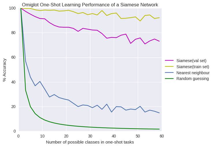
As shown in the figure, the accuracy on the validation set is slightly lower than that on the training set, especially when the number of N is large, which definitely indicates an overfitting problem. We also want to test how traditional regularization methods (like dropout) perform when the validation set is completely different from the training set. For larger N, it performed better than I expected, maintaining around 65% average accuracy with 50-60 categories.

Discussion

Now we have just trained a binary classification network to determine whether two images are the same or different. More importantly, we demonstrated that the model can perform one-shot learning on 20 classes of unseen alphabets. Of course, this is not the only way to perform one-shot learning using deep learning.

As I mentioned earlier, I think the biggest flaw of this Siamese network is that it has to compare the test image with each image in the training set one by one. When this network compares the test image with any image x1, regardless of what the training set is, is the same. This is silly; if you are performing a one-shot learning task, you see an image that is very similar to the test image. However, when you see another image in the training set that is also very similar to the test set, you will be less confident about its category. The training target and the test target are different; if there is a model that can compare the test image with the training set well while having the restriction of only one training image of the same category, the model would perform better.

The paper Matching Networks for One Shot Learning does exactly this. They use a deep model to learn a complete nearest neighbor classifier end-to-end, rather than learning a similarity function, training directly on one-shot tasks instead of on a pair of images. Andrej Karpathy’s notes explain this issue very well. Since you are learning machine classification, you can view it as meta-learning.

The paper One-Shot Learning with Memory-Augmented Neural Networks explains the relationship between one-shot learning and meta-learning; it trained a memory-augmented network on the Omniglot dataset. However, I admit I do not understand this paper.

What’s Next?

The Omniglot dataset is from 2015, and now there are scalable machine learning algorithms that have reached human-level performance on specific one-shot learning tasks. I hope that one day the Omniglot dataset will become a standard benchmark for one-shot learning, just as MNIST is for supervised learning.

Image classification is cool, but I do not think it is the most interesting problem in the machine learning community. Now that we know deep one-shot learning has achieved good results, I think it would be really cool to try to apply one-shot learning to more challenging tasks.

The idea of one-shot learning can be applied to sample-efficient reinforcement learning, especially in problems like OpenAI’s Universe, which has many Markov decision processes or environments with similar visual and dynamic information. If there is a reinforcement learning mechanism that can effectively explore new environments after learning in a manner similar to Markov decision processes, that would be incredibly cool.

OpenAI’s Bit World

“One-Shot Imitation Learning” is my favorite one-shot learning paper. Its goal is to establish a mechanism that can learn robust strategies to solve a task after one human demonstration. It does this by:

1. Building a neural network that can map the current state and a sequence of states (human demonstrations) to an action;

2. Training this model on human demonstration actions and slightly varied tasks, aiming for the model to reproduce the second demonstration action based on the first demonstration.

This shocked me, providing a broad avenue for creating learnable robots that can be widely applied.

Introducing one-shot learning into NLP is also a cool idea. Matching Networks have attempted this on one-shot language models, filling in missing words on the test set with just a small training set, and it seems to work well. Awesome!

Conclusion

In conclusion, thank you for reading! I hope you have grasped the concept of one-shot learning through one-shot learning. If not, I would be happy to hear your feedback and questions.

Original article link: https://sorenbouma.github.io/blog/oneshot/

[Extra] New Intelligence is conducting a new round of recruitment, flying to the most beautiful spaceship in the intelligent universe, with N seats left.

Click to read the original text for job details, looking forward to your joining!