
Author: Wu Xiaoyi Column Author of Python Enthusiasts Community
Personal Blog: Wu Xiaoyi
Zhihu Profile: Wu Xiaoyi丶
WeChat Official Account: Data Road (shuju_lu)
Code and Data Acquisition Method: Follow the WeChat Official Account “Python Enthusiasts Community” and reply:Practical Mining
This article is the practical part of the book “Python Data Analysis and Mining Practical”,整理分析后的复现. This article is the practical part of Chapter 6 of the book: Automatic Identification of Electricity Theft Users.
Table of Contents
I. Background and Mining Objectives
1.1 Background
1.2 Objectives
II. Analysis Methods and Processes
2.1 Analysis Methods
2.2 Process Organization
2.3 Data Exploration
2.4 Data Preprocessing
1. Electricity Consumption Trend Decrease Indicator
2. Line Loss Indicator
3. Model Construction
2.5 Model Comparison and Evaluation
2.6 Conducting Electricity Theft Diagnosis
III. Summary
I. Background and Mining Objectives
1.1 Background
1. Traditional methods for preventing electricity theft mainly rely on regular inspections, periodic verification of electric meters, and user reports of theft to detect theft or meter malfunctions.
2. However, this method is heavily dependent on human resources and lacks clear targets for theft detection.
3. By collecting information such as abnormal electricity consumption, abnormal load, terminal alarms, main station alarms, and abnormal line losses, a data analysis model is established to monitor electricity theft in real time and detect meter malfunctions.
1.2 Objectives
1. To summarize the key characteristics of electricity theft users and construct an identification model for them.
2. To utilize real-time detection data to call the electricity theft user identification model for real-time diagnosis.
II. Analysis Methods and Processes
2.1 Analysis Methods
1. Electricity theft users account for only a small portion of the monitored large users in the automated power measurement system, and certain large users, such as banks, tax offices, schools, and businesses, cannot exhibit theft behavior. Therefore, it is necessary to exclude these user categories during data preprocessing.
2. The electricity load in the system does not directly reflect the theft behavior of users, and terminal alarms often have many false positives and missed reports. Thus, data exploration and preprocessing are required to summarize the behavioral patterns of electricity theft users and extract feature indicators describing them from the data.
3. Finally, by combining historical information of electricity theft users, an expert sample dataset for the identification model is organized, and a classification model is further constructed to achieve automatic identification of electricity theft users. The identification process for electricity theft users is shown in Figure 6.1 and includes the following steps.
2.2 Process Organization
1. Selectively extract raw data from the automated power measurement system and marketing system, including electricity load, terminal alarms, and penalties for theft from a portion of large users.
2. Conduct exploratory analysis on the sample data, excluding users from industries that cannot exhibit electricity theft behavior, i.e., whitelist users, and preliminarily examine the electricity consumption characteristics of normal and theft users.
3. Preprocess the sample data, including data cleaning, handling missing values, and data transformation.
4. Construct an expert sample set.
5. Construct an electricity theft user identification model.
6. Monitor user electricity loads and terminal alarms online, and call the model to achieve real-time diagnosis.
2.3 Data Exploration
The following code can be used to open the dataset directly in Excel for graphical analysis.
2.3.1 Distribution Analysis
2.3.2 Periodic Analysis
2.3.3 Electricity Theft Consumption Analysis
2.4 Data Preprocessing
2.4.1 Data Cleaning
1. Non-residential users do not exhibit leakage, such as schools, post offices, etc.
2. Considering business, public holidays tend to be lower than usual, so to achieve better results, we remove holidays.
2.4.2 Handling Missing Values
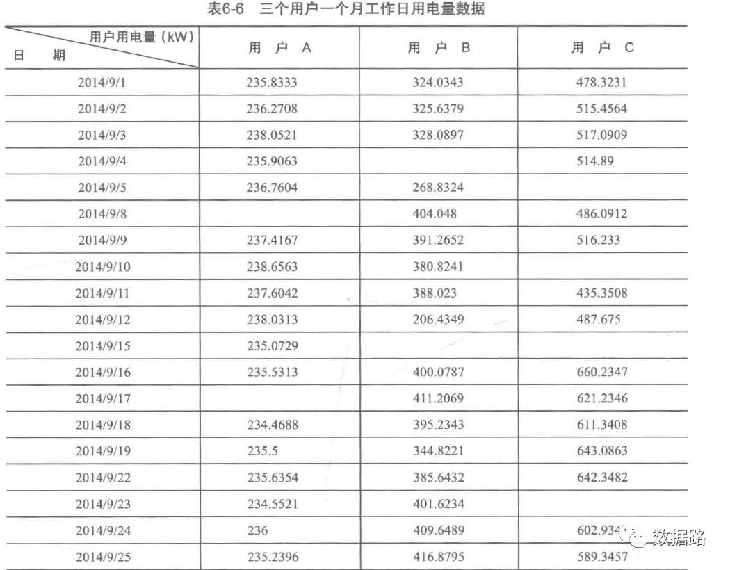
See the dataset content for details.
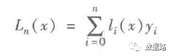
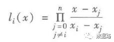
For handling missing values, the Lagrange interpolation method is used, as follows.
1. First, determine the independent and dependent variables in the original dataset,
2. Extract five data points before and after the missing value (remove empty and non-existent values),
3. Extract ten data points as a group and use the Lagrange polynomial interpolation formula.
#-*- coding: utf-8 -*-
# Lagrange interpolation code
import pandas as pd # Import data analysis library Pandas
from scipy.interpolate import lagrange # Import Lagrange interpolation function

inputfile = '/home/kesci/input/date14037/missing_data.xls' # Input data path, needs to be in Excel format;
outputfile = '/home/kesci/work/missing_data_processed.xls' # Output data path, needs to be in Excel format, here on Kesci, so local running needs to modify the path

data = pd.read_excel(inputfile, header=None) # Read data
print(data)
# Custom column vector interpolation function
# s is the column vector, n is the position to be interpolated, k is the number of data points taken before and after, default is 5
def ployinterp_column(s, n, k=5):
  y = s[list(range(n-k, n)) + list(range(n+1, n+1+k))] # Take data, note that this type of () takes the leftmost, does not take the rightmost.
  y = y[y.notnull()] # Remove empty values
  return lagrange(y.index, list(y))(n) # Interpolate and return the interpolation result

# Check each element to see if interpolation is needed
for i in data.columns:
  for j in range(len(data)):
    if (data[i].isnull())[j]: # If empty, interpolate.
      data[i][j] = ployinterp_column(data[i], j)

print(data)
data.to_excel(outputfile, header=None, index=False) # Output results

           0         1         2
0   235.8333  324.0343  478.3231
1   236.2708  325.6379  515.4564
2   238.0521  328.0897  517.0909
3   235.9063       NaN  514.8900
4   236.7604  268.8324       NaN
5        NaN  404.0480  486.0912
6   237.4167  391.2652  516.2330
7   238.6563  380.8241       NaN
8   237.6042  388.0230  435.3508
2.4.3 Data Transformation
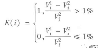
Although the electricity and load data collected from the power measurement system can reflect certain patterns of user theft behavior to some extent, they are not obvious enough to serve as expert samples for model construction and need to be reconstructed. Based on data transformation, new evaluation indicators are obtained to characterize the patterns of theft behavior, and the evaluation indicator system is shown in Figure 6巧.
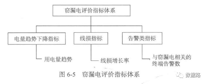
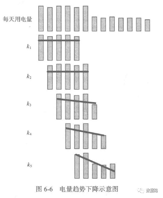
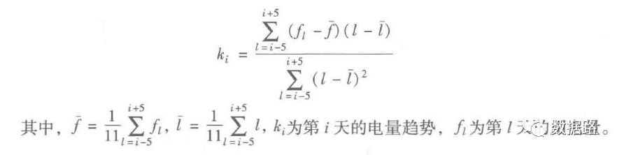
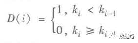
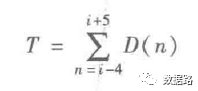
1. Electricity Consumption Trend Decrease Indicator
From the previous periodic analysis, it can be seen that the electricity consumption of theft users tends to decline continuously and then stabilize. Normal users, overall, show a stable trend. Therefore, it is considered to fit a line for a period of electricity consumption and calculate the indicator based on the slope.
2. Line Loss Indicator
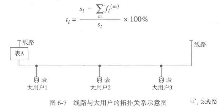
Based on the above indicator calculation methods, data is obtained. For details, see the model.xls in the dataset. If you want to ask me how to calculate the numbers, I am also confused. I will find an opportunity to learn the mathematical formula calculation methods and then supplement the corresponding code. However, I think it can be handled relatively simply and quickly using Excel. The expert sample data used for training can be found in the attached model.xls
2.5 Model Construction
2.5.1 Constructing the Electricity Theft User Identification Model
1. Data Division
For the expert sample, randomly select 20% as the test sample and 80% as the training sample. The code is as follows:
2. LM Neural Network
Using the Keras library to establish our neural network model, set the input nodes of the LM neural network to 3, output nodes to 1, and hidden nodes to 10, using the Adam method for solving, and using Relu(x)=max(x,0) as the activation function for the hidden layer. Experimental results show that this function can significantly improve the accuracy of the model.
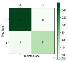
The following code takes two to three minutes to run, and upon completion, a confusion matrix chart is obtained. It can be calculated that the classification accuracy is (161+58)/(161+58+6+7)=94.4%, the normal users misclassified as electricity theft users account for 7/(161+7)=4.2%, and the electricity theft users misclassified as normal users account for 6/(6+58)=9.4%.
#-*- coding: utf-8 -*-
import matplotlib.pyplot as plt
import pandas as pd
from random import shuffle

def cm_plot(y, yp):
  from sklearn.metrics import confusion_matrix # Import confusion matrix function
  cm = confusion_matrix(y, yp) # Confusion matrix
  import matplotlib.pyplot as plt # Import plotting library
  plt.matshow(cm, cmap=plt.cm.Greens) # Plot confusion matrix, color scheme uses cm.Greens, more styles can be found on the official website.
  plt.colorbar() # Color label
  for x in range(len(cm)): # Data labels
    for y in range(len(cm)):
      plt.annotate(cm[x,y], xy=(x, y), horizontalalignment='center', verticalalignment='center')
  plt.ylabel('True label') # Axis label
  plt.xlabel('Predicted label') # Axis label
  return plt

datafile = '/home/kesci/input/date14037/model.xls'
data = pd.read_excel(datafile)
data = data.as_matrix()
shuffle(data)

p = 0.8 # Set training data ratio
train = data[:int(len(data)*p),:]# Slicing method for multi-dimensional data
test = data[int(len(data)*p):,:]# The left side of the comma represents rows, and the right side represents columns

# Build LM neural network model
from keras.models import Sequential # Import neural network initialization function
from keras.layers.core import Dense, Activation # Import neural network layer function, activation function

netfile = '/home/kesci/input/date14037/net.model' # Path to save the constructed neural network model

net = Sequential() # Establish neural network
net.add(Dense(input_dim = 3, output_dim = 10)) # Add connection from input layer (3 nodes) to hidden layer (10 nodes)
net.add(Activation('relu')) # Use relu activation function for hidden layer
net.add(Dense(input_dim = 10, output_dim = 1)) # Add connection from hidden layer (10 nodes) to output layer (1 node)
net.add(Activation('sigmoid')) # Use sigmoid activation function for output layer
net.compile(loss = 'binary_crossentropy', optimizer = 'adam') # Compile model, using adam method to solve

net.fit(train[:,:3], train[:,3], nb_epoch=100, batch_size=1) # Train model, loop 1000 times, not used in book source code, here need to delete class value to run normally
net.save_weights(netfile) # Save model

predict_result = net.predict_classes(train[:,:3]).reshape(len(train)) # Predict results reshape
''' Here it should be noted that keras uses predict to give the predicted probability, predict_classes gives the predicted category, and both prediction results are n x 1 dimensional arrays, not the usual 1 x n '''

# Import the custom confusion matrix visualization function, see the code cm_plot(y, yp) at the top
cm_plot(train[:,3], predict_result).show() # Show confusion matrix visualization result

from sklearn.metrics import roc_curve # Import ROC curve function

predict_result = net.predict(test[:,:3]).reshape(len(test))
fpr, tpr, thresholds = roc_curve(test[:,3], predict_result, pos_label=1)
plt.plot(fpr, tpr, linewidth=2, label = 'ROC of LM') # Plot ROC curve
plt.xlabel('False Positive Rate') # Axis label
plt.ylabel('True Positive Rate') # Axis label
plt.ylim(0,1.05) # Boundary range
plt.xlim(0,1.05) # Boundary range
plt.legend(loc=4) # Legend
plt.show() # Show plot results
The following are the running results, which can be viewed on Kesci during the training process.
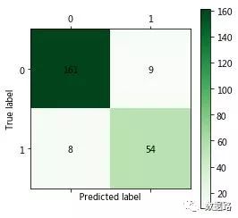
Model evaluation and analysis: The LM neural network uses the Keras library to establish the neural network model, setting the input nodes of the LM neural network to 3, output nodes to 1, and hidden nodes to 10, using the Adam method for solving, and using Relu(x)=max(x,0) as the activation function for the hidden layer. Experimental results show that this function can significantly improve the accuracy of the model.
The above code takes two to three minutes to run, and upon completion, a confusion matrix chart is obtained. It can be calculated that the classification accuracy is (161+58)/(161+58+6+7)=94.4%, the normal users misclassified as electricity theft users account for 7/(161+7)=4.2%, and the electricity theft users misclassified as normal users account for 6/(6+58)=9.4%.
3. CART Decision Tree Algorithm
#-*- coding: utf-8 -*-
# Build and test CART decision tree model

import pandas as pd # Import data analysis library
from random import shuffle # Import random function shuffle, used to shuffle data

datafile = '/home/kesci/input/date14037/model.xls' # Data name
data = pd.read_excel(datafile) # Read data, the first three columns are features, the fourth column is the label
data = data.as_matrix() # Convert table to matrix
shuffle(data) # Randomly shuffle data

p = 0.8 # Set training data ratio
train = data[:int(len(data)*p),:] # The first 80% is the training set
test = data[int(len(data)*p):,:] # The last 20% is the test set


# Build CART decision tree model
from sklearn.tree import DecisionTreeClassifier # Import decision tree model

treefile = '/home/kesci/work/tree.pkl' # Model output name
tree = DecisionTreeClassifier() # Establish decision tree model
tree.fit(train[:,:3], train[:,3]) # Train

# Save model
from sklearn.externals import joblib
joblib.dump(tree, treefile)

# Import the custom confusion matrix visualization function

def cm_plot(y, yp):
  from sklearn.metrics import confusion_matrix # Import confusion matrix function
  cm = confusion_matrix(y, yp) # Confusion matrix
  import matplotlib.pyplot as plt # Import plotting library
  plt.matshow(cm, cmap=plt.cm.Greens) # Plot confusion matrix, color scheme uses cm.Greens, more styles can be found on the official website.
  plt.colorbar() # Color label

  for x in range(len(cm)): # Data labels
    for y in range(len(cm)):
      plt.annotate(cm[x,y], xy=(x, y), horizontalalignment='center', verticalalignment='center')

  plt.ylabel('True label') # Axis label
  plt.xlabel('Predicted label') # Axis label
  return plt

cm_plot(train[:,3], tree.predict(train[:,:3])).show() # Show confusion matrix visualization result
# Note that Scikit-Learn uses the predict method to directly give the prediction result.


from sklearn.metrics import roc_curve # Import ROC curve function

fpr, tpr, thresholds = roc_curve(test[:,3], tree.predict_proba(test[:,:3])[:,1], pos_label=1)
plt.plot(fpr, tpr, linewidth=2, label = 'ROC of CART', color = 'green') # Plot ROC curve
plt.xlabel('False Positive Rate') # Axis label
plt.ylabel('True Positive Rate') # Axis label
plt.ylim(0,1.05) # Boundary range
plt.xlim(0,1.05) # Boundary range
plt.legend(loc=4) # Legend
plt.show() # Show plot results
The running results are as follows:
Model evaluation and analysis: The classification accuracy is (160+56)/(160+56+3+13)=93.1%, and the obtained confusion matrix is shown above. Because each random sample is different, the random accuracy fluctuates within a certain range.
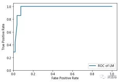
Model Comparison and Evaluation
Using the ROC curve evaluation method, an excellent classifier should have a ROC curve that is as close to the upper left corner as possible.
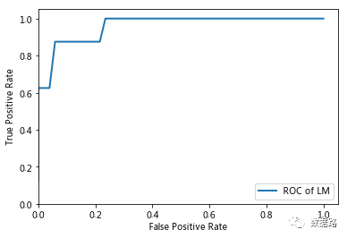
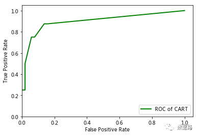
By comparison, it can be easily concluded that the ROC curve of the LM neural network is more in line with the definition of excellence, indicating that the classification performance of the LM neural network model is good and can be applied to the identification of electricity theft users.
3. Conducting Electricity Theft Diagnosis
Monitor user electricity loads and terminal alarm data online, and use the model obtained from Section 2.3 to input online real-time data, then use the previously constructed electricity theft user identification model to calculate the diagnosis results of users’ electricity theft, achieving real-time diagnosis of electricity theft users.
III. Summary
1. Gained an understanding of the practical applications of LM neural network and CART decision tree algorithms in data mining.
2. However, a deep understanding of the principles behind these two algorithms has not yet been achieved, which needs to be comprehended while learning “Introduction to Data Mining” in the future.
3. Understood the ROC comparison method in evaluating the strengths and weaknesses of identification models, but there should be better methods.
4. This case can be extrapolated to projects related to tax evasion in automobiles. However, during practical operations, it was found that it is difficult to identify effective indicators and establish evaluation metrics from the original target data, and the ability to understand business transformations is insufficient.
5. Currently, I am also learning Qin Lu’s “Seven Weeks Data Analyst” hoping to gain some business capabilities to assist with the project.

Historical Articles Collection of Python Enthusiasts Community:
Historical article list of Python Enthusiasts Community (updated weekly)
 Benefits: Scan the QR code at the end of the article to immediately follow the WeChat Official Account,“Python Enthusiasts Community”, and start learning Python courses:
After following, reply in the official account“Course” to obtain:
The editor’s introductory video course on Python!!!
Teacher Cui’s web scraping practical cases free learning video.
Teacher QiuIntroduction to Data Sciencefree learning video.
Teacher Chen’s Data Analysis Report Production free learning video.
Master big data analysis! Spark 2.X + Python essence practical coursefree learning video.
Teacher Qiu’s Python web scraping practical free learning video.