Comprehensive Summary of Machine Learning Basics

Machine learning is divided into two main categories based on model types: supervised learning models and unsupervised learning models.

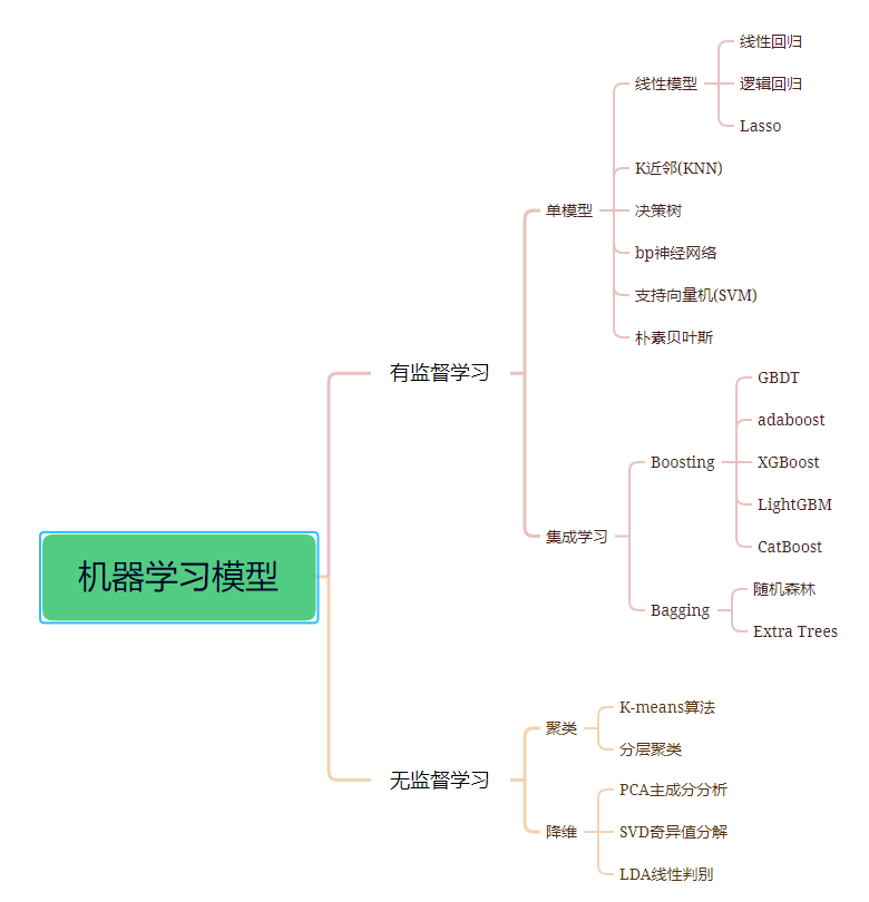
1. Supervised Learning

Supervised learning typically uses training data with expert-labeled tags to learn a function mapping from input variable X to output variable Y. Y = f(X), and the training data is usually in the form of (n×x, y), where n represents the size of the training sample, and x and y are the sample values of variables X and Y, respectively.

Supervised learning can be divided into two categories:

• Classification problems: Predicting the category of a sample (discrete). For example, determining gender, health status, etc.
• Regression problems: Predicting the corresponding real number output (continuous) of a sample. For example, predicting the average height of people in a certain area.

Additionally, ensemble learning is also a type of supervised learning. It combines the predictions of multiple relatively weak machine learning models to predict new samples.

1.1 Single Model

1.11 Linear Regression

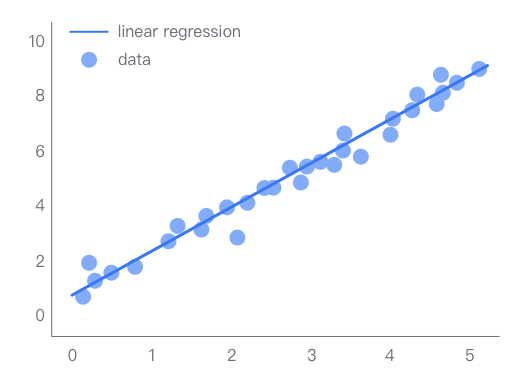
Linear regression refers to a regression model composed entirely of linear variables. In linear regression analysis, only one independent variable and one dependent variable are included, and their relationship can be approximately represented by a straight line; this type of regression analysis is called simple linear regression analysis.

If the regression analysis includes two or more independent variables, and there is a linear relationship between the dependent variable and the independent variables, it is called multiple linear regression analysis.

1.12 Logistic Regression

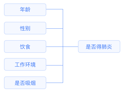
Used to study the influence relationship between X and Y when Y is categorical data. If Y has two categories, such as 0 and 1 (e.g., 1 for willing and 0 for not willing, 1 for purchase and 0 for no purchase), it is called binary logistic regression; if Y has three or more categories, it is called multi-class logistic regression.

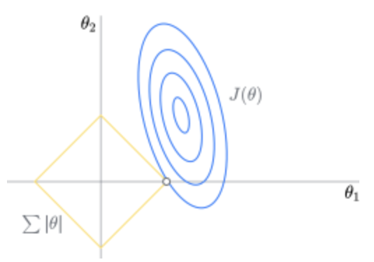
The independent variables do not necessarily have to be categorical; they can also be quantitative variables. If X is categorical data, dummy variable coding is required for X.

1.13 Lasso

The Lasso method is a compression estimation method that replaces the least squares method. The basic idea of Lasso is to establish an L1 regularization model, during which some coefficients are compressed and some coefficients are set to zero. Once the model training is complete, the parameters with weights equal to 0 can be discarded, making the model simpler and effectively preventing overfitting. It is widely used for fitting and variable selection in the presence of multicollinearity data.

1.14 K-Nearest Neighbors (KNN)

The main difference between KNN for regression and classification lies in the decision-making process during the final prediction. For classification predictions, KNN generally uses the majority voting method, meaning it predicts the class of the sample based on the majority class among the K nearest samples in the training set.

For regression, KNN typically uses the average method, taking the average output of the K nearest samples as the regression prediction value. However, their theories are the same.

1.15 Decision Tree

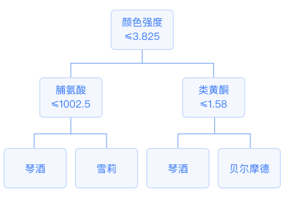
In a decision tree, each internal node represents a splitting problem: it specifies a test on a certain attribute of the instance, splitting the samples reaching that node according to a specific attribute, and each successor branch of that node corresponds to a possible value of that attribute.

The leaf nodes of the classification tree contain samples where the output variable’s mode is the classification result. The leaf nodes of the regression tree contain samples where the output variable’s mean is the predicted result.

1.16 BP Neural Network

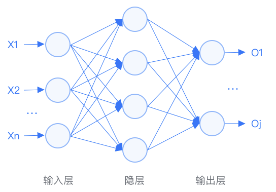
The BP neural network is a multi-layer feedforward network trained by the error backpropagation algorithm and is one of the most widely used neural network models. The learning rule of the BP neural network uses the steepest descent method to continuously adjust the network’s weights and thresholds through backpropagation, minimizing the classification error rate (minimizing the sum of squared errors).

BP neural networks are multi-layer feedforward neural networks characterized by: signals are propagated forward, while errors are propagated backward. Specifically, for a neural network model with only one hidden layer, the BP neural network process is mainly divided into two stages:

• The first stage is the forward propagation of signals from the input layer through the hidden layer to the output layer;
• The second stage is the backward propagation of errors from the output layer to the hidden layer and finally to the input layer, adjusting the weights and biases from the hidden layer to the output layer and from the input layer to the hidden layer in turn.

1.17 Support Vector Machine (SVM)

Support Vector Machine Regression (SVR) uses nonlinear mapping to map data into a high-dimensional feature space, allowing the independent and dependent variables to have good linear regression characteristics in that space. After fitting in that feature space, it returns to the original space.

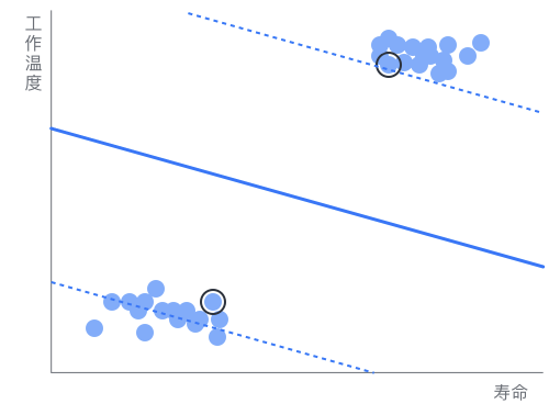
Support Vector Machine Classification (SVM) is a type of generalized linear classifier that performs binary classification of data using supervised learning methods, with the decision boundary being the maximum margin hyperplane solved from the learning samples.

1.18 Naive Bayes

Given the premise of one event occurring, calculate the probability of another event occurring — we will use Bayes’ theorem. Assuming prior knowledge is d, to calculate the probability that our hypothesis h is true, we will use the following Bayes’ theorem:

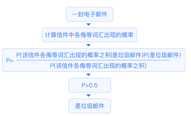
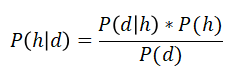
This algorithm assumes that all variables are independent of each other.

1.2 Ensemble Learning

Ensemble learning is a method that combines the results of different learning models (such as classifiers) to further improve accuracy through voting or averaging. Generally, voting is used for classification problems, and averaging is used for regression problems. This approach is based on the idea that “many hands make light work”.

Ensemble algorithms mainly fall into three categories: Bagging, Boosting, and Stacking. This article will not discuss stacking.

• Boosting

1.21 GBDT

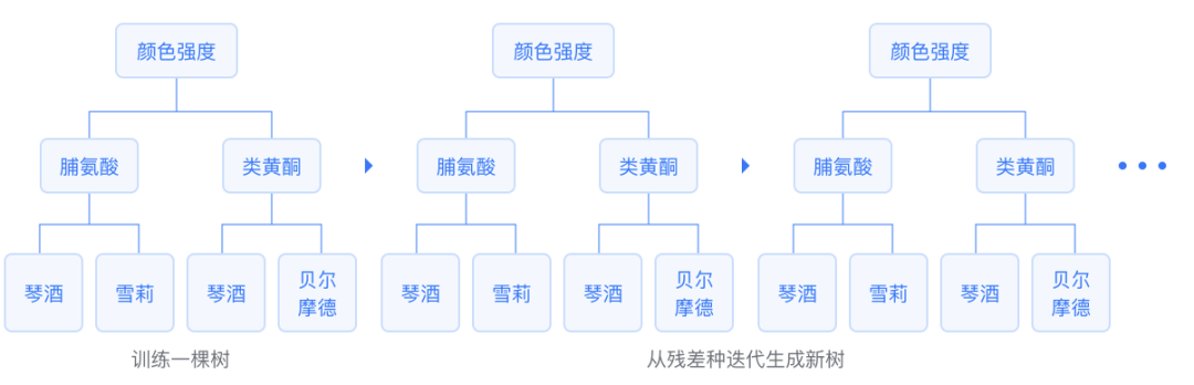
GBDT is a Boosting algorithm that uses CART regression trees as base learners. It is an additive model that serially trains a set of CART regression trees, ultimately summing the predictions of all regression trees to obtain a strong learner, where each new tree fits the negative gradient direction of the current loss function. The final output is the sum of this set of regression trees, directly yielding regression results or applying the sigmoid or softmax function to obtain binary or multi-class classification results.

1.22 AdaBoost

AdaBoost assigns a high weight to learners with low error rates and a low weight to learners with high error rates, combining weak learners with corresponding weights to generate a strong learner. The difference between regression and classification algorithms lies in the way error rates are calculated; classification problems generally use a 0/1 loss function, while regression problems generally use a squared loss function or a linear loss function.

1.23 XGBoost

XGBoost stands for “Extreme Gradient Boosting”. The XGBoost algorithm is a type of composite algorithm formed by combining base functions with weights to achieve good fitting effects on the data. Due to its strong generalization ability, high scalability, and fast computation speed, XGBoost has been popular in statistics, data mining, and machine learning since its introduction in 2015.

XGBoost is an efficient implementation of GBDT. Unlike GBDT, XGBoost adds a regularization term to the loss function; and since some loss functions are difficult to derive, XGBoost uses the second-order Taylor expansion of the loss function for fitting.

1.24 LightGBM

LightGBM is an efficient implementation of XGBoost, which discretizes continuous floating-point features into k discrete values and constructs a histogram with a width of k. It then traverses the training data to calculate the cumulative statistics of each discrete value in the histogram. During feature selection, it only needs to find the optimal split point based on the discrete values of the histogram and uses a leaf-wise growth strategy with depth restrictions, saving considerable time and space costs.

1.25 CatBoost

CatBoost is a GBDT framework based on symmetric decision tree algorithms, mainly addressing the pain points of efficiently and reasonably handling categorical features and dealing with gradient bias and prediction shift issues to improve the accuracy and generalization ability of the algorithm.

• Bagging

1.26 Random Forest

Random forest classification generates numerous decision trees by randomly sampling both the observational data set and the feature variables. Each sampling result corresponds to one tree, and each tree generates its own rules and classification results (judgment values). The forest ultimately integrates all decision trees’ rules and classification results (judgment values) to implement the classification (regression) of the random forest algorithm.

1.27 Extra Trees

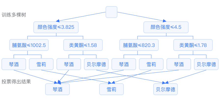
Extra Trees (Extremely Randomized Trees) is very similar to random forests. The term “extremely random” refers to the random feature and threshold partitioning in decision trees, resulting in greater shape and difference variability in each decision tree.

2. Unsupervised Learning

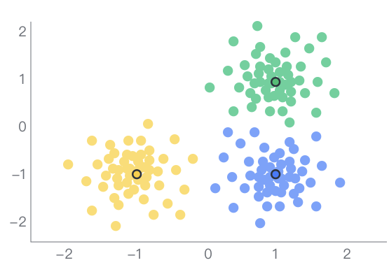
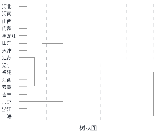
Unsupervised learning deals with training data that only has input variables X without corresponding output variables. It models the structure of the data without expert-labeled training data.

2.1 Clustering

Clustering divides similar samples into a cluster. Unlike classification problems, clustering problems do not know the categories in advance, and naturally, the training data does not have category labels.

2.11 K-means Algorithm

Clustering analysis is a center-based clustering algorithm (K-means clustering) that iteratively assigns samples to K classes, minimizing the sum of distances between each sample and the center or mean of its assigned class. Unlike hierarchical clustering algorithms that cluster based on fields, fast clustering analysis clusters based on samples.

2.12 Hierarchical Clustering

Hierarchical clustering is a type of clustering that performs hierarchical decomposition of a given set of data objects. Hierarchical clustering algorithms build clusters layer by layer, forming a tree with clusters as nodes. If the decomposition is done from the bottom up, it is called agglomerative hierarchical clustering, such as AGNES. If the decomposition is done from the top down, it is called divisive hierarchical clustering, such as DIANA. The most commonly used method is agglomerative hierarchical clustering.

2.2 Dimensionality Reduction

Dimensionality reduction refers to reducing the dimensions of data while preserving meaningful information. Using feature extraction methods and feature selection methods can achieve dimensionality reduction. Feature selection refers to selecting a subset of the original variables, while feature extraction transforms data from high dimensions to low dimensions. The widely known principal component analysis algorithm is a method of feature extraction.

2.21 PCA Principal Component Analysis

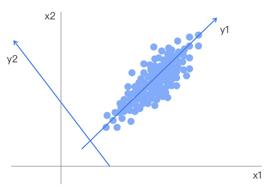
Principal component analysis linearly combines multiple correlated indicators to explain as much information as possible from the original data with the least dimensions. The resulting variables after dimensionality reduction are linearly independent of each other, and the newly determined variables are linear combinations of the original variables, with the later principal components having a smaller weight in variance, indicating weaker capacity for summarizing original information.

2.22 SVD Singular Value Decomposition

Singular Value Decomposition (SVD) is an algorithm widely used in the field of machine learning. It can be used not only in feature value decomposition in dimensionality reduction algorithms but also in recommendation systems and natural language processing, serving as the foundation for many algorithms.

2.23 LDA Linear Discriminant Analysis

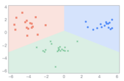
The principle of linear discriminant analysis is to project samples onto a line such that the projection points of similar samples are as close as possible, while the projection points of different samples are as far apart as possible. When classifying new samples, they are projected onto the same line, and their class is determined based on the position of their projection points.

This article is from SPSSPRO, providing a comprehensive summary of machine learning knowledge points. It is recommended to bookmark it for slow reading, as the full text is divided into detailed algorithm explanations of supervised and unsupervised learning!

If you like it, feel free to bookmark, like, and share it!

Edit / Zhang Zhihong

Review / Fan Ruiqiang

Recheck / Zhang Zhihong

Click below

Follow us

Read the original text