Today is the seventh issue summarizing 16 major topics and 124 interview questions in machine learning: K-Nearest Neighbors (KNN) algorithm interview questions.
The K-Nearest Neighbors (KNN) algorithm works by finding the K nearest neighbors of a sample and using the information from these K neighbors to make predictions. For classification tasks, the majority voting method is usually employed, meaning the predicted class is the majority class among the K nearest neighbors; for regression tasks, it typically uses the average of the neighbors.
The “nearness” in KNN is defined through distance metrics (such as Euclidean distance, Manhattan distance, etc.).
It is an instance-based learning algorithm that does not require a training phase; all computations are performed during the prediction phase.
Some Advantages
-
Simple and Understandable: The algorithm’s logic is straightforward, making it easy to understand and implement. -
No Training Required: There is no explicit learning process, saving training time. -
Adaptive: Theoretically capable of predicting for any distribution of data. -
Versatile: Can be used for classification, regression, and even recommendation systems.
Some Disadvantages
-
Computationally Intensive: For each test sample, distances must be computed for all training samples, resulting in a high computational load. -
High Storage Requirements: All training data must be retained. -
Curse of Dimensionality: In high-dimensional spaces, distance metrics may become ineffective, leading to performance degradation. -
Sensitive to Imbalanced Data: In datasets with imbalanced class distributions, minority classes may be overlooked.
Suitable Application Scenarios
-
Small-scale Datasets: Performs well on small to medium-sized datasets where computational load is manageable. -
Baseline Model: Commonly used as a baseline method for quick implementation and performance comparison. -
Real-time Decision Making: Due to its instance-based learning characteristics, it is suitable for real-time decision systems needing dynamic model updates. -
Low-dimensional Data: Best suited for low to medium-dimensional data, performing poorly on high-dimensional data.
In summary, KNN performs well on small to medium-sized, low-dimensional, and class-balanced datasets and can serve as an initial exploration method for many problems.
The old rule: If you find recent articles good, feel free to like and share them, so more friends can see them.
K-Nearest Neighbors Algorithm Interview Questions List
1. What is the K-Nearest Neighbors algorithm? How does it perform classification and regression?
2. What does the K value in KNN represent? How to choose an appropriate K value?
3. How does KNN handle distance metrics for features? What are the common distance measurement methods?
4. What are the limitations of KNN? Under what circumstances might it be unsuitable?
5. What are the time and space complexities of the KNN algorithm? How are they affected by dataset size and dimensions?
Next, I will elaborate on each interview question in detail~~~~
01
1. What is the K-Nearest Neighbors algorithm? How does it perform classification and regression?
K-Nearest Neighbors (KNN) is a fundamental machine learning algorithm commonly used for classification and regression problems.
The working principle is simple and can be summarized in the following steps:
1. Training Phase: During the training phase, the algorithm stores all training sample data and their corresponding classes or labels.
2. Testing Phase: In the testing phase, for a sample to be classified or regressed, the algorithm finds the K nearest training samples.
3. Classification: For classification problems, the KNN algorithm uses the most common class among these K nearest training samples to predict the class of the sample to be classified. For example, if K=3, and these three nearest training samples belong to classes A, B, and B, then the sample to be classified will be predicted as class B.
4. Regression: For regression problems, the KNN algorithm uses the average or weighted average of the K nearest training samples to predict the output of the sample to be regressed. For instance, if K=3, and the target values of these three nearest training samples are 5, 6, and 7, then the output of the sample to be regressed will be predicted as their average or weighted average.
An example of implementing the KNN algorithm using Python:
from sklearn.neighbors import KNeighborsClassifier

# Create training dataset
X_train = [[1, 2], [2, 3], [3, 1], [6, 7], [7, 8], [8, 6]]
y_train = ['A', 'A', 'A', 'B', 'B', 'B']

# Create KNN classifier object, set K=3
knn = KNeighborsClassifier(n_neighbors=3)

# Train KNN classifier
knn.fit(X_train, y_train)

# Create sample to classify
X_test = [[4, 5], [9, 10]]

# Predict the class of the sample to classify
y_pred = knn.predict(X_test)

print(y_pred)  # Output: ['A' 'B']
In the above example, we first created a training dataset X_train and corresponding class labels y_train. Then, we created a KNN classifier object using the KNeighborsClassifier class and set the K value to 3. Next, we trained the KNN classifier by calling the fit method.
After that, we created the sample to classify X_test and used the trained KNN classifier to predict it, obtaining the predicted class labels y_pred. Finally, we output the prediction results, which show that the samples to be classified are predicted to belong to classes ‘A’ and ‘B’.
2. What does the K value in KNN represent? How to choose an appropriate K value?
In the K-Nearest Neighbors (KNN) algorithm, the K value represents the number of nearest neighbors to consider. The basic principle of KNN is that when given a new sample point, it searches for the K nearest neighbors in the training set and classifies or regresses based on these neighbors’ labels.
Choosing an appropriate K value is crucial as it affects the performance and accuracy of the KNN algorithm. Here are some common methods to select a suitable K value:
1. Rule of Thumb: According to the rule of thumb, generally selecting a smaller K value can reduce the impact of noise, but it may also lead to overfitting. A larger K value can smooth the decision boundary but may be affected by irrelevant data. Common K values typically range from 1 to 10.
2. Cross-validation: Use cross-validation to select the best K value. Divide the training set into K subsets, then perform KNN classification on each subset, calculating prediction accuracy or other evaluation metrics. By cross-validating at different K values, select the K value that yields the best model performance.
3. Consider Dataset Size: For smaller datasets, a smaller K value is usually better to avoid overfitting. For larger datasets, a larger K value can be chosen.
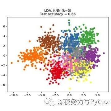
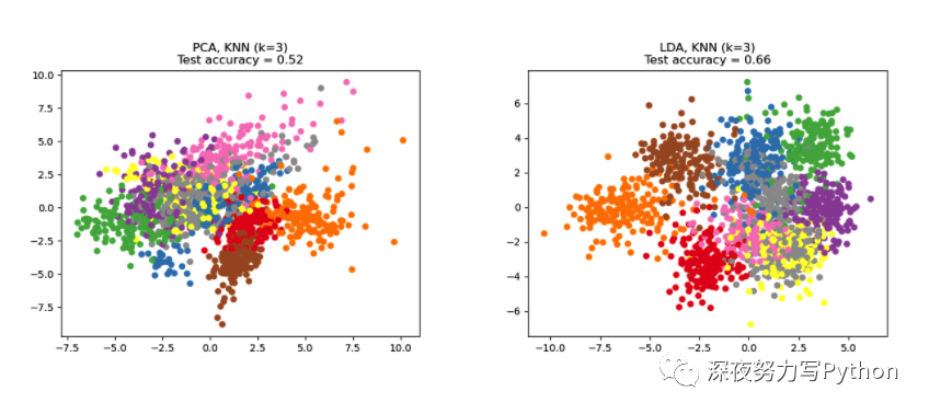
4. Visualization and Analysis: Visualizing and analyzing the data can help choose the appropriate K value. By trying different K values and observing changes in the decision boundary, you can determine which K values fit the data better.
It is important to note that selecting an appropriate K value is an empirical task, depending on the characteristics of the dataset and the specific application scenario. Therefore, when using the KNN algorithm, it is often necessary to try different K values and evaluate their performance to select the best one.
3. How does KNN handle distance metrics for features? What are the common distance measurement methods?
For more details, see here: link
The KNN algorithm measures the similarity between samples by calculating the distances, which are then used for classification or regression. Common distance measurement methods include the following:
1. Euclidean Distance: The Euclidean distance is the most commonly used distance measurement method. For two sample points x and y, their Euclidean distance in an n-dimensional feature space can be represented as:
4. What are the limitations of KNN? Under what circumstances might it be unsuitable?
5. What are the time and space complexities of the KNN algorithm? How are they affected by dataset size and dimensions?
-
Distance Calculation: For each test sample, the KNN algorithm needs to calculate the distance between the new sample and all training samples. This step’s time complexity depends on the size of the dataset N and the number of features D. Specifically, the time complexity for distance calculation is O(N * D). -
Sorting: After finding the K nearest neighbors, the KNN algorithm needs to sort these neighbors to determine the final prediction. The time complexity for sorting is typically O(K * log(K)). -
Prediction: The time complexity for prediction for each test sample is O(1).
-
Storing Training Set: The KNN algorithm needs to keep all training samples in memory for predictions. Therefore, its space complexity equals the size of the training set multiplied by the number of features, i.e., O(N * D).
-
The Impact of Dataset Size: As the training set size N increases, the required storage space will also grow linearly.
-
The Impact of Dataset Dimensions: As the number of features D increases, the space required to store the training set will also increase.
Machine Learning Interview Summary List
Finally
Recommended Reading
sklearn handling supervised learning algorithm case summary!
sklearn handling unsupervised learning algorithm case summary!
sklearn series (I) decision tree case summary!
sklearn series (II) matrix decomposition and dimensionality reduction issues!
sklearn series (III) classification algorithm case summary!!