Deep Learning: Structured Machine Learning Projects

When you have built a machine learning system and obtained some preliminary results, a lot of improvements are often needed to achieve the most satisfactory results. As mentioned in the previous optimization of neural networks, there are various methods for improvement, which may involve collecting more data, performing regularization, or adopting different optimization algorithms.

To accurately find the direction for improvement and make a machine learning system work faster and more effectively, it’s essential to learn some commonly used strategies in building machine learning systems.

One of the challenges in building a machine learning system is that there are many things to try and change. For example, there are many hyperparameters that need to be tuned. It is crucial to grasp the direction of trials and changes and recognize the impact of each adjustment made.

Orthogonalization is a system design attribute that ensures that modifying an algorithm instruction or component in a system does not produce or propagate side effects to other components in the system.

It makes it easier to validate one algorithm independently of another, while also reducing design and development time.

For example, when learning to drive a car, you primarily learn the three basic control methods: steering, acceleration, and braking. These three control methods do not interfere with each other; you only need to practice continuously to master them.

However, if you were to learn to drive a car with only one joystick that controls a certain angle and speed with each operation, the learning cost would be much higher. This is the principle of orthogonalization.

When designing a supervised learning system, you need to meet the following four assumptions, and they should be orthogonal:

1. The established model performs well on the training set;

2. The established model performs well on the development set (validation set);

3. The established model performs well on the test set;

4. The established model performs well in real-world applications.

Once orthogonalization is achieved, if you find:

1. Performance on the training set is not good enough — try using a deeper neural network or switching to a better optimization algorithm;

2. Performance on the development set is not good enough — try regularization or adding more training data;

3. Performance on the test set is not good enough — try using more of the development set for testing validation;

4. Performance in real applications is not good enough — it may be because the test set was not set correctly or the cost function evaluation was incorrect.

When facing various issues, orthogonalization can help us pinpoint and effectively solve problems.

When building a machine learning system, by setting a single-number evaluation metric, you can quickly determine which of the different results obtained after several adjustments is better.

For a classifier, the metric used to evaluate its performance is generally the classification accuracy, which is the ratio of the number of correctly classified samples to the total number of samples. It can also serve as a single-number evaluation metric. For example, several algorithms of the previous cat classifier were evaluated based on accuracy.

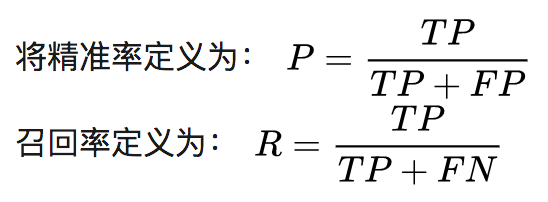
Common evaluation metrics for binary classification problems are precision and recall, where the class of interest is treated as positive and all others as negative. The classifier predicts correctly or incorrectly, with four possible outcomes:

• TP (True Positive) — Number of positive predictions correctly identified

• FN (False Negative) — Number of positive predictions incorrectly identified

• FP (False Positive) — Number of negative predictions incorrectly identified as positive

• TN (True Negative) — Number of negative predictions correctly identified

When faced with situations that are difficult to judge, you need to use F1 Score to evaluate the performance of two classifiers.

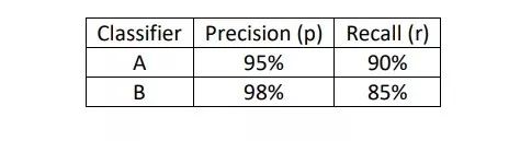
The F1 score is defined as:

The F1 score is actually the harmonic mean of precision and recall, which is an improvement method based on their average, yielding better results than simply taking the average.

Thus, the F1 score for classifier A in the above image is 92.4%, while that for classifier B is 91.0%, indicating that classifier A performs better. Here, the F1 score serves as a single-number evaluation metric.

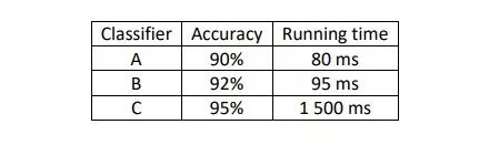
However, sometimes the evaluation criteria are not limited to a single-number metric. For example, in the case of several cat classifiers shown above, you may want to care about both their recognition accuracy and runtime. But combining these two metrics into a single-number metric is not ideal.

In this case, you need to set one metric as an optimizing metric and others as satisficing metrics.

In the previous example, accuracy is an optimizing metric because you want the classifier to classify correctly as much as possible, while runtime is a satisficing metric. If you want the classifier’s runtime to not exceed a certain value, then the classifier you should choose is the one with the highest accuracy within that runtime limit, thus making a trade-off.

In addition to using these criteria to evaluate a model, you should also learn to adjust some evaluation metrics in a timely manner when necessary, or even change the training data.

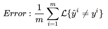
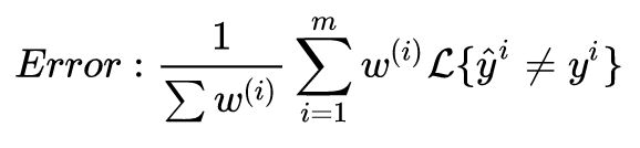
For instance, if classifiers A and B have recognition errors of 3% and 5% respectively, but for some reason, classifier A misclassifies pornographic images as cats, causing user discomfort, while B does not have this issue, then classifier B, despite having a larger error, may actually be the better classifier. You can calculate the false recognition rate using the following formula:

You can also set a weight ω⁽ⁱ⁾ such that when x⁽ⁱ⁾ is a pornographic image, ω⁽ⁱ⁾ is 10, otherwise it is 1, to differentiate pornographic images from other misidentified images:

Thus, it is essential to correctly determine an evaluation metric based on the actual situation to ensure that this metric is optimal.

When building a machine learning system, the method of handling the dataset will affect the progress of the entire building process. As previously mentioned, the collected existing data is generally divided into training set, development set, and test set, with the development set also referred to as the cross-validation set.

When building a machine learning system, different methods are employed to train different models on the training set, and then the development set is used to evaluate the models’ performance. When a model is deemed sufficiently effective, it is tested using the test set.

First, it is important to note that the sources of the development set and the test set must be the same and must be randomly sampled from all data. The selected development and test sets should also be as consistent as possible with the real data that the machine learning system will face in the future to minimize deviation from the target.

Next, attention should be paid to the size division of each dataset. In the early days of machine learning, for all the data you had, it was common to use 70% as the training set and the remaining 30% as the test set; or if a development set was included, 60% as the training set and 20% each for development and test sets.

This division was reasonable when the obtained data was relatively small. However, in today’s machine learning era, where data is typically in the thousands or more, traditional data division methods cannot be applied.

If you have obtained one million data samples, using 98% as the training set and only 1% (i.e., ten thousand data) as the development set and 1% as the test set is sufficient.

Therefore, data division should be based on the actual situation rather than rigidly adhering to tradition.

The size of the test set should be set sufficiently to enhance the credibility of the overall system performance, and the size of the development set should also be set sufficiently to evaluate several different models.

Today, designing and establishing a machine learning system has become simpler and more efficient than before, and some machine learning algorithms can now match human performance in many fields, such as the globally renowned AlphaGo developed by Google DeepMind.

However, many tasks that we humans can complete nearly perfectly are still being attempted to be matched or surpassed by machine learning systems.

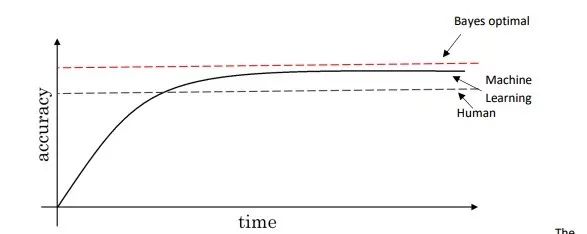
The above image shows the changes in performance levels of machine learning and humans over time. Generally, when machine learning exceeds human performance levels, its progress slows down significantly. One important reason for this is that human performance on certain natural perception problems approaches Bayes Error.

Bayes Error is defined as the optimal possible error; in other words, no mapping function from x to accuracy y can exceed this value.

When the performance of the established machine learning model has not yet reached human performance levels, various methods can be employed to enhance it. For example, training with manually labeled data, conducting error analysis to understand why humans can recognize correctly, or performing variance and bias analysis.

The concepts of bias and variance were previously discussed in optimizing neural networks. By comparing the performance level of a machine learning model with human performance on a task, you can clearly indicate the quality of the model’s performance and determine whether to reduce bias or variance in subsequent work.

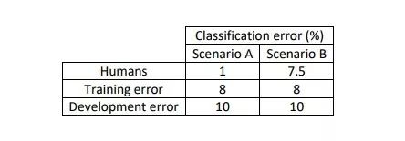
The difference between the training set error and human performance level error is called avoidable bias.

For example, in the two scenarios depicted in the image above, comparing the error rates of humans and machine learning models shows that in scenario A, the learning algorithm’s error rate and the human’s error rate have a significant avoidable bias. In this case, subsequent work should focus on reducing the training set’s error rate to minimize bias. In scenario B, the learning algorithm’s performance is comparable to that of humans, with an avoidable bias of only 0.5%, so future efforts should shift towards minimizing the variance in the development and training sets, which is at 2%.

Human performance levels provide a way to estimate Bayes error. When training a machine learning system for a specific task, using human performance levels on that task as the Bayes error helps avoid optimizing the training process with a target error rate of 0%.

Therefore, when obtaining human error data for a task, these data can be used as a proxy for Bayes error to analyze the bias and variance of the learning algorithm.

If the error difference between the training set and human performance level is greater than that between the training set and development set, future efforts should focus on reducing bias; conversely, efforts should focus on reducing variance.

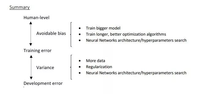
The image above summarizes various methods to address bias and variance. In summary, a small avoidable bias indicates that the model’s training process is well-executed, while an acceptable level of variance suggests that the established model performs equally well on the development and test sets as it does on the training set.

Furthermore, if the avoidable error is negative, indicating that the machine learning model’s performance exceeds the human performance level (the proxy for Bayes error), it does not mean that your model’s performance has reached its peak. To further improve its performance, alternative optimization methods must be sought.

Today, machine learning has achieved this in many fields, such as online advertising, product promotion, predicting logistics transport times, credit assessment, and more.

Note: The images and materials referenced in this article are organized and translated from Andrew Ng’s Deep Learning series courses, with all rights reserved. The translation and organization may have limitations; please feel free to point out any inaccuracies.

Recommended Reading:

Markov Decision Process: Markov Processes

【Deep Learning Practice】How to Handle Variable Length Sequences Padding in PyTorch

【Basic Theory of Machine Learning】Detailed Explanation of Maximum A Posteriori Probability Estimation (MAP)