

Hello everyone, welcome to the Moon Inn, I am the shopkeeper Kong Character.
The content directory for this issue is as follows. If this content helps you, feel free to like and share to support the shopkeeper! If you also recognize the column content of the inn, please click here to become a co-creator of the inn.
-
Chapter 8 Temporal and Model Fusion -
8.1 TextCNN Network -
8.1.1 TextCNN Structure -
8.1.2 Text Segmentation -
8.1.3 TextCNN Implementation -
8.1.4 Summary -
References
Chapter 8 Temporal and Model Fusion
After the introduction of the content in Chapters 4 and 7, we have a clear understanding of two common network structures in deep learning: CNN and RNN. CNN is mainly used to process feature data with dependencies in spatial positions, while RNN is mainly used to handle feature data with temporal dependencies. Nevertheless, we can still extract features from temporal data using either CNN or a combination of CNN and RNN. In this chapter, we will introduce various variant models based on CNN and RNN along with corresponding application cases.
8.1 TextCNN Network
Although CNN is primarily used for feature encoding of information at adjacent spatial positions in the input matrix, it can also characterize the feature information of temporal data in a sequence using multi-scale convolutional windows, such as the classic TextCNN[1] text classification model. The core idea of TextCNN is to represent each word with a fixed-length vector (i.e., word vector, which will be introduced in section 9.2); then, the word vectors of all words in a sentence are stacked vertically to form a matrix, where the number of words in the sentence is represented, and the dimension of the word vector is indicated; finally, a fixed-width multi-scale convolution kernel is used for feature extraction and subsequent tasks.
8.1.1 TextCNN Structure
TextCNN uses convolution operations to extract local features from the text, capturing local features of different lengths with convolution kernels of varying sizes, thereby identifying key information in the text. In TextCNN, the entire network model is generally divided into three layers: convolutional layer, pooling layer, and fully connected classification layer, as shown in Figure 8-1.
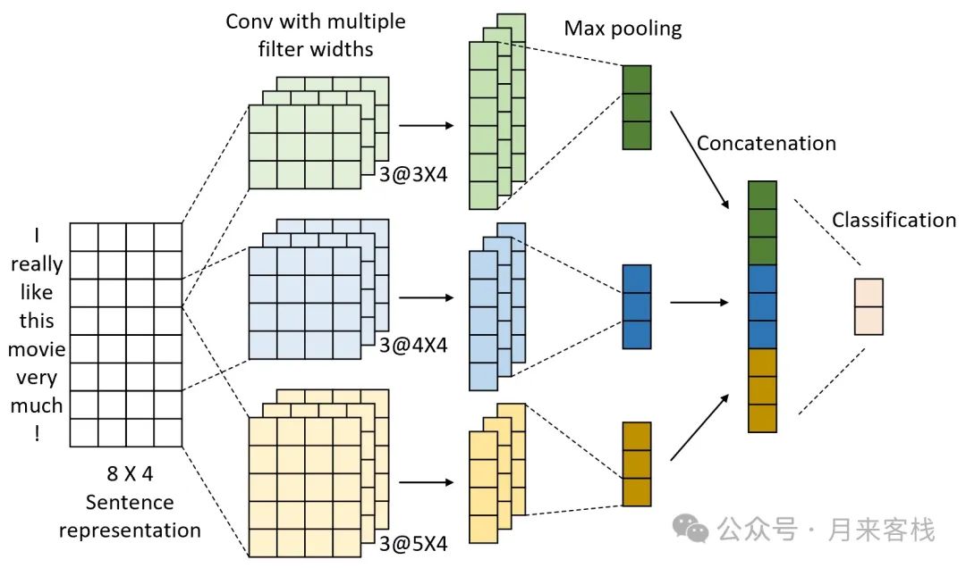
In Figure 8-1, the leftmost part is a feature matrix, where each row is a 4-dimensional vector, with each vector representing a fixed word from the vocabulary. Based on this representation method, any text can be represented as a fixed-width feature matrix, which can be viewed as a single-channel feature map. Furthermore, TextCNN employs three convolution kernels of different window lengths (3, 4, and 5) for convolution processing. At this point, since the width of the convolution kernel is consistent with the width of the feature map, the output after convolution is a one-dimensional vector. It can be seen that this convolution operation can essentially be viewed as a feature extraction process for local sequential information in the text, with the length depending on the window length of the convolution kernel.
After completing the convolution operation, a max pooling operation is performed on each feature map to extract features, resulting in each channel becoming a scalar value. Finally, all results are concatenated to obtain a vector as the feature representation of the text, followed by a classification layer to complete subsequent classification tasks. Although the TextCNN network structure seems relatively simple, it often achieves good results in practical applications, with fast training speeds and low risks of overfitting.
8.1.2 Text Segmentation
In section 7.6, we used a single character granularity along with a word embedding layer to represent text. Next, we will see how to represent text using word granularity and a word embedding layer. Of course, if it is English corpus, there is no distinction between characters and words.
Text segmentation refers to dividing a sentence from a Chinese semantic perspective to obtain smaller word units. For example, for the following text:
“To Live” is a novel by Yu Hua, depicting the hardships and resilience of Chinese farmers. Through the protagonist Fugui’s life experiences, it showcases the devastation caused by war, hunger, and political movements on the people, while conveying profound reflections on family, hope, and humanity.
The result after segmentation is:
《/活着/》/是/余华/的/小说/,/描绘/了/中国/农民/的/苦难/与/坚韧/。/通过/主人公/福贵/的/生活/经历/,/展现/了/战乱/、/饥饿/和/政治/运动/对/人民/的/摧残/,/同时/传递/了/关于/家庭/、/希望/和/人性/的/深刻/思考/。
Then, word frequency statistics are conducted at the word level to construct a vocabulary and vectorize the text.
In text processing, jieba is a commonly used open-source segmentation tool[3], which can be installed via the command pip install jieba. Meanwhile, the jieba library provides two segmentation modes to handle Chinese segmentation in different scenarios, which will be introduced below.
1. Standard Segmentation Mode
The standard segmentation mode refers to the conventional method of segmenting a sentence into multiple words, with the following example code:
1 import jieba
2 if __name__ == '__main__':
3     sen = "The weather is clear today, the sun is shining, and a gentle breeze is caressing my face as I stroll alone along the river path."
4     segs = jieba.cut(sen)
5     result = "/".join(segs)
In the above code, line 4 performs segmentation on the original text and returns an iterator. Line 5 formats the processed result, as shown below.
今天/天气晴朗/,/阳光明媚/,/微风/轻拂/着/脸庞/,/我/独自/漫步/在/河边/的/小径/上/。2. Full Segmentation Mode
Although the above method can complete the segmentation of a sentence at the word level, some words can have different segmentation methods. In this case, you can specify the full segmentation mode in the cut function by using jieba.cut(sen, cut_all=True) to obtain all possible segmentation results. For example, after enabling the full segmentation mode, the segmentation result is:
今天/今天天气/天天/天气/天气晴朗/晴朗/,/阳光/阳光明媚/光明/明媚/,/微风/轻拂/着/脸庞/,/我/独自/漫步/在/河边/的/小径/上/。In practice, you can choose different modes according to the situation. Of course, jieba not only performs segmentation but also provides functions for keyword extraction, part-of-speech tagging, and new word discovery, which interested readers can refer to for further study.
8.1.3 TextCNN Implementation
After understanding the principles related to the TextCNN model, let’s see how to quickly implement this model using PyTorch. The complete example code can be found in the Code/Chapter08/C01_TextCNN/TextCNN.py file.
1. Forward Propagation
First, we need to implement the entire forward propagation process of the model. As shown in Figure 8-1, the entire model is divided into four parts: word embedding layer, convolution layer, pooling layer, and fully connected layer. The implementation code is as follows:
 1 class TextCNN(nn.Module):
 2     def __init__(self, vocab_size=2000, embedding_size=512,
 3                  window_size=None, out_channels=2, fc_hidden_size=128, num_classes=10):
 4         super(TextCNN, self).__init__()
 5         if window_size is None:
 6             window_size = [3, 4, 5]
 7         self.vocab_size = vocab_size
 8         self.embedding_size = embedding_size
 9         self.window_size = window_size
10         self.out_channels = out_channels
11         self.fc_hidden_size = fc_hidden_size
12         self.num_classes = num_classes
13         self.token_embedding = nn.Embedding(self.vocab_size, self.embedding_size)
14         self.convs = [nn.Conv2d(1, out_channels,
15                       kernel_size=(k, embedding_size)) for k in window_size]
16         self.max_pool = nn.AdaptiveMaxPool2d((1, 1))
17         self.classifier = nn.Sequential(
18             nn.Linear(len(self.window_size) * self.out_channels, self.num_classes))
In the above code, lines 5-12 are for initializing relevant model hyperparameters. Line 13 instantiates a word embedding layer, which is a two-dimensional weight matrix where each row corresponds to a unique vector representation of each word in the vocabulary. Lines 14-15 instantiate multiple convolutional layers based on different convolution window lengths. Line 16 instantiates an adaptive max pooling layer, whose output shape is [1,1], and since the pooling layer has no parameters, multiple convolutional layers can share the same pooling layer. Lines 17-18 instantiate a classification layer, with the input dimension equal to the number of convolution layers multiplied by the number of output channels of each convolution layer.
Furthermore, the example code for the entire forward propagation calculation process is as follows:
 1     def forward(self, x, labels=None):
 2         x = self.token_embedding(x)
 3         x = torch.unsqueeze(x, dim=1)
 4         features = []
 5         for conv in self.convs:
 6             feature = self.max_pool(conv(x))
 7             features.append(feature.squeeze(-1).squeeze(-1))
 8         features = torch.cat(features, dim=1)
 9         logits = self.classifier(features)
10         if labels is not None:
11             loss_fct = nn.CrossEntropyLoss(reduction='mean')
12             loss = loss_fct(logits, labels)
13             return loss, logits
14         else:
15             return logits
In the above code, line 1 x is the index representation of each sentence after segmentation in the vocabulary, with a shape of [batch_size, src_len]. Line 2 is the result after processing through the word embedding layer, with an output shape of [batch_size, src_len, embedding_size]. Line 3 indicates that x is expanded in the first dimension, resulting in a shape of [batch_size, 1, src_len, embedding_size]. Lines 4-7 perform multi-scale convolution operations, where line 6 shows that the shape after convolution and pooling is [batch_size, out_channels, 1, 1], and line 7 compresses the dimensions to [batch_size, out_channels] and stores them in a list. Line 8 combines all features, resulting in a shape of [batch_size, out_channels*len(window_size)]. Line 9 is the final classification layer. Lines 10-15 return the corresponding processing results based on conditions.
Finally, it can be used as follows:
1 if __name__ == '__main__':
2     x = torch.tensor([[1, 2, 3, 2, 0, 1],
3                       [2, 2, 2, 1, 3, 1]])
4     labels = torch.tensor([0, 3])
5     model = TextCNN(vocab_size=5, embedding_size=3, fc_hidden_size=6)
6     loss, logits = model(x, labels)
7     print(logits.shape)
The output is:
1 torch.Size([2, 10])2. Constructing the Dataset
Here, we will continue to use the Toutiao 15 classification dataset mentioned in section 7.2.4, just needing to change the granularity from character level to word level. Specifically, we need to add a new segmentation processing logic to the tokenize function in the TouTiaoNews module introduced in section 7.2.4, with the example code as follows:
1 def tokenize(text, cut_words=False):
2     if cut_words:
3         text = jieba.cut(text)
4     words = " ".join(text).split()
5     return words
In the above code, lines 2-3 are the newly added segmentation processing logic.
Furthermore, we only need to pass the cut_words parameter to the places in TouTiaoNews where the tokenize function is used to construct the dataset at the word level, and the specific example code can be found directly in the source code. The vectorized samples are similar to the following results:
1 ## Original input sample: Will traveling to Yunnan cause altitude sickness, and how to prevent it?
2 ## Segmented sample: ['去', '云南', '旅行', '会', '不会', '出现', '高原', '反应', ',', '应', '如何', '预防', '?']
3 ## Vectorized sample: [60, 1220, 391, 29, 196, 317, 0, 2368, 2, 1343, 15, 0, 3]
Finally, when instantiating TouTiaoNews, we just need to pass cut_words=True:
1 if __name__ == '__main__':
2     toutiao_news = TouTiaoNews(top_k=4000,batch_size=12,cut_words=True)
3     test_iter = toutiao_news.load_train_val_test_data(is_train=False)
4     for x,y in test_iter:
5         print(x,y)
3. Model Training
As this part of the code has been introduced multiple times before, I will not elaborate here. Readers can directly refer to the source code. Finally, during the training of the network model, similar output results will be obtained:
 1 Epochs[1/50]--batch[0/2093]--Acc: 0.0469--loss: 2.775
 2 Epochs[1/50]--batch[50/2093]--Acc: 0.2109--loss: 2.4728
 3 Epochs[1/50]--batch[100/2093]--Acc: 0.3203--loss: 2.229
 4 Epochs[1/50]--batch[150/2093]--Acc: 0.4453--loss: 1.7122
 5 Epochs[1/50]--batch[200/2093]--Acc: 0.5156--loss: 1.5143
 6 Epochs[1/50]--batch[250/2093]--Acc: 0.5547--loss: 1.2475
 7 Epochs[1/50]--batch[300/2093]--Acc: 0.5859--loss: 1.5477
 8 Epochs[1/50]--batch[350/2093]--Acc: 0.6172--loss: 1.2619
 9 Epochs[1/50]--batch[400/2093]--Acc: 0.6953--loss: 1.146
10 Epochs[1/50]--Acc on val 0.7311
8.1.4 Summary
In this section, we first introduced the principles of TextCNN in detail, which can essentially be viewed as a method for local feature extraction from sequential data using convolution operations; then we briefly introduced the usage of the segmentation tool jieba; finally, we showed how to implement the TextCNN model step by step and tested it on the Toutiao dataset. In the next section, we will introduce the RNN-based TextRNN model for text classification.
References
[1] Kim Y. 2014. Convolutional Neural Networks for Sentence Classification [C]. In Proceedings of the 2014 Conference on EMNLP, pages 1746–1751.
[2] Zhang Y, Wallace B. A sensitivity analysis of (and practitioners’ guide to) convolutional neural networks for sentence classification[J]. arXiv preprint, 2015, arXiv:1510.03820.
[3] https://github.com/fxsjy/jieba