Hello everyone, I am Red Stone!
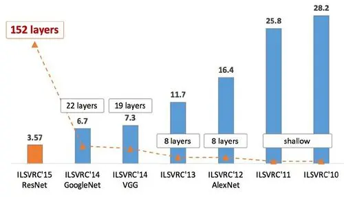
The first typical CNN is the LeNet5 network, while the first CNN to shine brightly was AlexNet. In 2012, AlexNet emerged in the globally renowned image recognition competition ILSVRC, directly reducing the error rate by nearly 10 percentage points, which was something all previous machine learning models could not achieve.
The authors of AlexNet are Alex Krizhevsky and others from the University of Toronto. Alex Krizhevsky is a student of Hinton. It is popular online to say that Hinton, LeCun, and Bengio are the three giants in the field of neural networks, with LeCun being the author of LeNet5 (Yann LeCun).
Before formally introducing AlexNet, let’s briefly talk about what this network is used for. Similar to LeNet-5, AlexNet is also a convolutional neural network for image recognition. The architecture of AlexNet is more complex with more parameters. In the ILSVRC competition, the dataset used by AlexNet is ImageNet, which recognizes a total of 1000 categories.
The paper titled ImageNet Classification with Deep Convolutional Neural Networks
Paper link:
http://www.cs.toronto.edu/~fritz/absps/imagenet.pdf
1. Network Structure
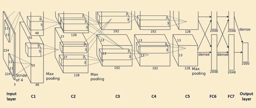
The overall network structure of AlexNet includes: 1 input layer, 5 convolutional layers (C1, C2, C3, C4, C5), 2 fully connected layers (FC6, FC7), and 1 output layer. Below is a detailed introduction to the network structure.
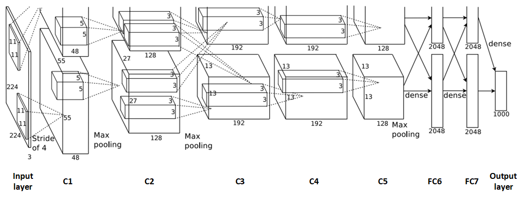
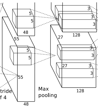
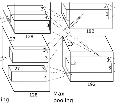
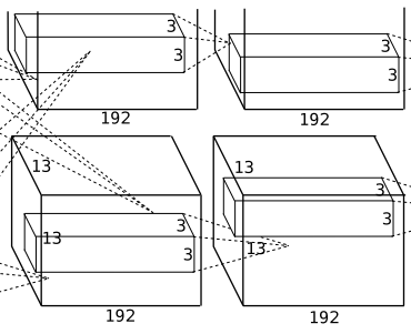
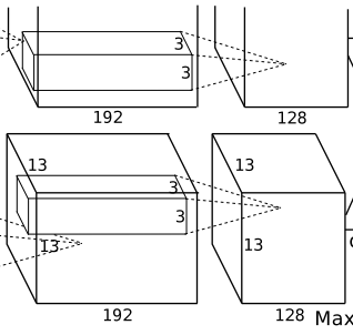
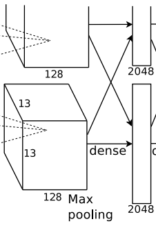
This image shows the structure of AlexNet. At first glance, some readers may wonder if the upper part of the network is not fully drawn. In fact, it is not. Due to the hardware resource limitations at that time, AlexNet’s complex structure and large number of parameters made it difficult to train on a single GPU. Therefore, AlexNet used two GTX 580 3GB GPUs for parallel training. This means that the original convolutional layers were split into two parts, with FeatureMaps trained on two GPUs (for example, the convolution layer 55x55x96 is split into two FeatureMaps: 55x55x48). The upper and lower parts in the image are symmetrical, so the upper part is not completely drawn.
It is worth mentioning that the convolution kernels in convolutional layers C2, C4, and C5 are only connected to the FeatureMap of the previous layer located on the same GPU, while the convolution kernels in C3 are connected to the FeatureMaps of the previous layers on both GPUs.
1.1 Input Layer
In the original paper, the input image size for AlexNet is 224x224x3. However, the actual image size is 227x227x3. It is said that 224×224 might have been a typo when writing the paper, or was it later adjusted for the network?
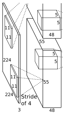
1.2 Convolutional Layer (C1)
The processing flow of this layer is: Convolution –> ReLU –> Local Response Normalization (LRN) –> Pooling.
Convolution: The input is 227x227x3, using 96 convolution kernels of size 11x11x3 for convolution, padding=0, stride=4. According to the formula: (input_size + 2 * padding – kernel_size) / stride + 1 = (227 + 2*0 – 11) / 4 + 1 = 55, the output is 55x55x96.
ReLU: The FeatureMap output from the convolution layer is input to the ReLU function.
Local Response Normalization: Local Response Normalization (LRN) is a technique to improve accuracy in deep learning. It is generally performed after activation and pooling. LRN creates a competitive mechanism for the activity of local neurons, making the larger responding values relatively larger and suppressing the smaller responding neurons, enhancing the generalization ability of the model.
The formula for LRN is as follows:
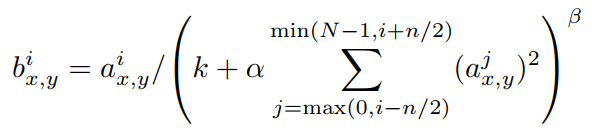
a is the neuron before normalization, b is the neuron after normalization; N is the number of convolution kernels, which is also the number of generated FeatureMaps; k, α, β, n are hyperparameters, with values used in the paper being k=2, n=5, α=0.0001, β=0.75.
The output of local response normalization is still 55x55x96. It is divided into two groups, each with a size of 55x55x48, located on a single GPU.
Pooling: Using a 3×3 pooling unit with stride=2 for max pooling. Note that overlapping pooling is used here, meaning the stride is less than the size of the pooling unit. According to the formula: (55 + 2*0 – 3) / 2 + 1 = 27, each group gets an output of 27x27x48.
1.3 Convolutional Layer (C2)
The processing flow of this layer is: Convolution –> ReLU –> Local Response Normalization (LRN) –> Pooling.
Convolution: Both groups of inputs are 27x27x48, with each group using 128 convolution kernels of size 5x5x48 for convolution, padding=2, stride=1. According to the formula: (input_size + 2 * padding – kernel_size) / stride + 1 = (27 + 2*2 – 5) / 1 + 1 = 27, each group outputs 27x27x128.
ReLU: The FeatureMap output from the convolution layer is input to the ReLU function.
Local Response Normalization: Normalization is performed using parameters k=2, n=5, α=0.0001, β=0.75. Each group output remains 27x27x128.
Pooling: Using a 3×3 pooling unit with stride=2 for max pooling. Note that overlapping pooling is used here, meaning the stride is less than the size of the pooling unit. According to the formula: (27 + 2*0 – 3) / 2 + 1 = 13, each group gets an output of 13x13x128.
1.4 Convolutional Layer (C3)
The processing flow of this layer is: Convolution –> ReLU
Convolution: The input is 13x13x256, using 384 convolution kernels of size 3x3x256 for convolution, padding=1, stride=1. According to the formula: (input_size + 2 * padding – kernel_size) / stride + 1 = (13 + 2*1 – 3) / 1 + 1 = 13, the output is 13x13x384.
ReLU: The FeatureMap output from the convolution layer is input to the ReLU function. The output is split into two groups, each with a size of 13x13x192, located on a single GPU.
1.5 Convolutional Layer (C4)
The processing flow of this layer is: Convolution –> ReLU
Convolution: Both groups of inputs are 13x13x192, with each group using 192 convolution kernels of size 3x3x192 for convolution, padding=1, stride=1. According to the formula: (input_size + 2 * padding – kernel_size) / stride + 1 = (13 + 2*1 – 3) / 1 + 1 = 13, each group outputs 13x13x192.
ReLU: The FeatureMap output from the convolution layer is input to the ReLU function.
1.6 Convolutional Layer (C5)
The processing flow of this layer is: Convolution –> ReLU –> Pooling
Convolution: Both groups of inputs are 13x13x192, with each group using 128 convolution kernels of size 3x3x192 for convolution, padding=1, stride=1. According to the formula: (input_size + 2 * padding – kernel_size) / stride + 1 = (13 + 2*1 – 3) / 1 + 1 = 13, each group outputs 13x13x128.
ReLU: The FeatureMap output from the convolution layer is input to the ReLU function.
Pooling: Using a 3×3 pooling unit with stride=2 for max pooling. Note that overlapping pooling is used here, meaning the stride is less than the size of the pooling unit. According to the formula: (13 + 2*0 – 3) / 2 + 1 = 6, each group gets an output of 6x6x128.
1.7 Fully Connected Layer (FC6)
The flow of this layer is: (Convolution) Fully Connected –> ReLU –> Dropout (Convolution)
Fully Connected: The input is 6×6×256, using 4096 convolution kernels of size 6×6×256 for convolution. Since the size of the convolution kernel is exactly the same as the input size, each coefficient in the convolution kernel corresponds exactly to a pixel value in the input size. According to the formula: (input_size + 2 * padding – kernel_size) / stride + 1 = (6 + 2*0 – 6) / 1 + 1 = 1, the output is 1x1x4096. This layer is called the fully connected layer.
ReLU: The output of these 4096 neurons is processed through the ReLU activation function.
Dropout: Randomly disconnect certain connections of the neurons in the fully connected layer to prevent overfitting by not activating certain neurons. The 4096 neurons are also distributed across two GPUs for computation.
1.8 Fully Connected Layer (FC7)
The flow of this layer is: (Convolution) Fully Connected –> ReLU –> Dropout
Fully Connected: The input is 4096 neurons, and the output is also 4096 neurons (as set by the authors).
ReLU: The output of these 4096 neurons is processed through the ReLU activation function.
Dropout: Randomly disconnect certain connections of the neurons in the fully connected layer to prevent overfitting.
The 4096 neurons are also distributed across two GPUs for computation.
1.9 Output Layer
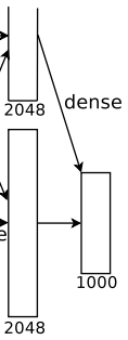
The flow of this layer is: (Convolution) Fully Connected –> Softmax
Fully Connected: The input is 4096 neurons, and the output is 1000 neurons. These 1000 neurons correspond to 1000 detection categories.
Softmax: The output of these 1000 neurons is processed through the Softmax function, outputting the predicted probability values for the 1000 categories.
2. Network Parameters
2.1 Number of Neurons in AlexNet
|
Layer |
Definition |
Quantity |
|
C1 |
Number of neurons in the FeatureMap of C1 layer |
55x55x48x2=290400 |
|
C2 |
Number of neurons in the FeatureMap of C2 layer |
27x27x128x2=186624 |
|
C3 |
Number of neurons in the FeatureMap of C3 layer |
13x13x192x2=64896 |
|
C4 |
Number of neurons in the FeatureMap of C4 layer |
13x13x192x2=64896 |
|
C5 |
Number of neurons in the FeatureMap of C5 layer |
13x13x128x2=43264 |
|
FC6 |
Number of neurons in the FC6 fully connected layer |
4096 |
|
FC7 |
Number of neurons in the FC7 fully connected layer |
4096 |
|
Output layer |
Number of neurons in the output layer |
1000 |
The total number of neurons in the AlexNet network is:
290400 + 186624 + 64896 + 64896 + 43264 + 4096 + 4096 + 1000 = 659272
Approximately 650,000 neurons.
2.2 Number of Parameters in AlexNet
|
Layer |
Definition |
Quantity |
|
C1 |
Convolution kernel 11x11x3, 96 convolution kernels, bias parameters |
(11x11x3+1)x96=34944 |
|
C2 |
Convolution kernel 5x5x48, 128 convolution kernels, 2 groups, bias parameters |
(5x5x48+1)x128x2=307456 |
|
C3 |
Convolution kernel 3x3x256, 384 convolution kernels, bias parameters |
(3x3x256+1)x384=885120 |
|
C4 |
Convolution kernel 3x3x192, 192 convolution kernels, 2 groups, bias parameters |
(3x3x192+1)x192x2=663936 |
|
C5 |
Convolution kernel 3x3x192, 128 convolution kernels, 2 groups, bias parameters |
(3x3x192+1)x128x2=442624 |
|
FC6 |
Convolution kernel 6x6x256, 4096 neurons, bias parameters |
(6x6x256+1)x4096=37752832 |
|
FC7 |
Fully connected layer, 4096 neurons, bias parameters |
(4096+1)x4096=16781312 |
|
Output layer |
Fully connected layer, 1000 neurons |
1000×4096=4096000 |
The total number of parameters in the AlexNet network is:
34944 + 307456 + 885120 + 663936 + 442624 + 37752832 + 16781312 + 4096000 = 60964224
Approximately 60 million parameters.
Assuming each parameter is a 32-bit floating point, each float is 4 bytes. Thus, the space occupied by the parameters is:
60964224 x 4 = 243856896(Byte) = 238141.5(Kb) = 232.56(Mb)
The parameters occupy approximately 232Mb of space.
2.3 FLOPs
FLOPS (Floating Point Operations Per Second) is a measure of computer performance, especially in fields that require a lot of floating point calculations. It is often used to estimate the execution efficiency of computers.
One MFLOPS (megaFLOPS) equals one million (10^6) floating point operations per second,
One GFLOPS (gigaFLOPS) equals one billion (10^9) floating point operations per second,
One TFLOPS (teraFLOPS) equals one trillion (10^12) floating point operations per second,
One PFLOPS (petaFLOPS) equals one quadrillion (10^15) floating point operations per second,
One EFLOPS (exaFLOPS) equals one quintillion (10^18) floating point operations per second.
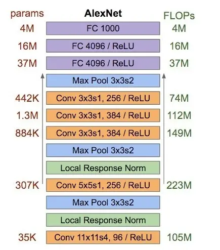
For the convolutional layers in the AlexNet network, FLOPS=num_params*(H*W). Where num_params is the number of parameters, H*W is the height and width of the convolution layer. For fully connected layers, FLOPS=num_params.
|
Layer |
Definition |
Quantity |
|
C1 |
num_params*(H*W) |
34944x55x55=105705600 |
|
C2 |
num_params*(H*W) |
307456x27x27=224135424 |
|
C3 |
num_params*(H*W) |
885120x13x13=149585280 |
|
C4 |
num_params*(H*W) |
663936x13x13=112205184 |
|
C5 |
num_params*(H*W) |
442624x13x13=74803456 |
|
FC6 |
num_params |
37752832 |
|
FC7 |
num_params |
16781312 |
|
Output layer |
num_params |
4096000 |
The overall structure of AlexNet, including the number of parameters and FLOPS of each layer, is shown in the following image:
3. Innovations of AlexNet
3.1 Data Augmentation
In this paper, the authors used two data augmentation methods:
-
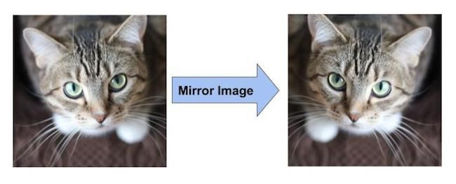
Mirror reflection and random cropping
-
Changing the intensity values of the RGB channels of training samples
The method of mirror reflection and random cropping is to first perform a mirror reflection on the image:
Then randomly crop a 227×227 region from the original image and the mirrored image (256×256):
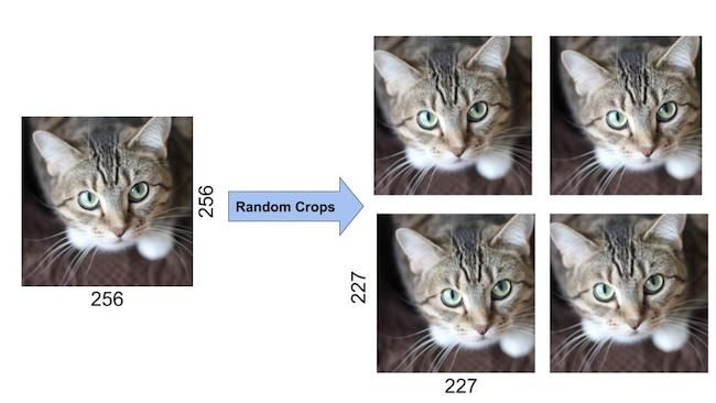
During testing, five crops were made from the top left, top right, bottom left, bottom right, and center, resulting in 10 crops, and then the results were averaged.
Changing the intensity values of the RGB channels of training samples involves performing PCA (Principal Component Analysis) on the RGB space, then applying a Gaussian perturbation of (0, 0.1) to the principal components, which changes color and lighting, resulting in a further 1% reduction in error rate.
3.2 Activation Function ReLU
At that time, the standard activation function for neurons was the tanh() function, which is a saturated nonlinear function and slower than non-saturated nonlinear functions during gradient descent. Therefore, AlexNet used the ReLU function as the activation function.
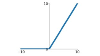
The ReLU function is a piecewise linear function that outputs 0 for inputs less than or equal to 0; for inputs greater than 0, it outputs the input itself. During backpropagation, for the part where ReLU has output, the derivative is always 1. Additionally, ReLU causes some neurons to output 0, leading to sparsity in the network and reducing the interdependence of parameters, mitigating overfitting issues.
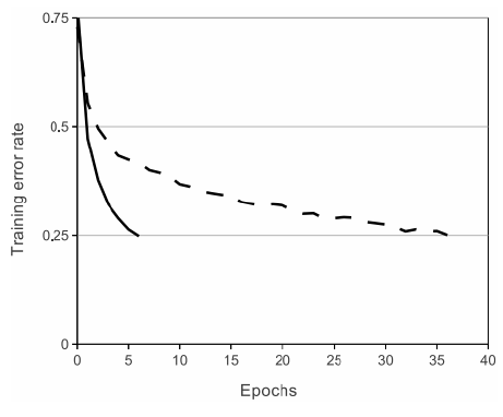
The following figure shows that using the ReLU function in a 4-layer convolutional network achieved a training error rate of 25% on the CIFAR-10 dataset 6 times faster than using the tanh function under the same conditions (the solid black line is using ReLU, the dashed black line is using tanh).
3.3 Local Response Normalization
Local Response Normalization (LRN) creates a competitive mechanism for the activity of local neurons, making the larger responding values relatively larger and suppressing the smaller responding neurons, enhancing the generalization ability of the model.
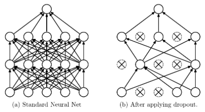
3.4 Dropout
Dropout is a commonly used method to suppress overfitting in neural networks. In neural networks, Dropout modifies the structure of the network itself. For the neurons of a certain layer, some neurons are set to 0 with a defined probability, meaning these neurons do not participate in forward and backward propagation, as if they were deleted from the network, while keeping the number of input and output neurons unchanged. Then, the parameters are updated according to the learning method of the neural network. In the next iteration, some neurons are randomly deleted again (set to 0) until training ends.
In the AlexNet network, the fully connected layers FC6 and FC7 used the Dropout method.
Dropout can be considered a significant innovation in AlexNet and is now a necessary structure in neural networks. Dropout can also be seen as a model ensemble, where each generated network structure is different, effectively reducing overfitting by combining multiple models. Dropout only requires twice the training time to achieve the effect of model averaging, making it very efficient.
3.5 Overlapping Pooling
Previously, average pooling layers were commonly used in CNNs, while AlexNet used max pooling layers exclusively. This avoided the blurring effect of average pooling layers, and since the stride is smaller than the size of the pooling kernel, the outputs of the pooling layers overlap, enhancing the richness of the features. Overlapping pooling can prevent overfitting, contributing to a 0.3% reduction in the Top-5 error rate.
3.6 Dual GPU Training
Due to the hardware limitations at the time, the authors of AlexNet used dual GPUs for training, which was an innovative engineering approach. Training with dual GPUs reduced the training time compared to single GPU networks, lowering the top-1 and top-5 error rates by 1.7% and 1.2%, respectively.
3.7 End-to-End Training
In the AlexNet network, the input to the CNN is directly an image, whereas at that time, many approaches involved using feature extraction algorithms to extract features from RGB images. AlexNet used an end-to-end network, where the only preprocessing of the image was subtracting the mean pixel values from the training set, without any other preprocessing of the image, directly using the RGB values of the pixels to train the network.
Hand-Crafted CNN Series:
Hand-Crafted CNN Classic Network: LeNet-5 (Theoretical Part)
Hand-Crafted CNN Classic Network: LeNet-5 (MNIST Practical Part)
Hand-Crafted CNN Classic Network: LeNet-5 (CIFAR10 Practical Part)
Hand-Crafted CNN Classic Network: LeNet-5 (Custom Practical Part)
If you find this article useful, please give it a thumbs up or share it on your friends’ circle!
Recommended Reading
(Clicking the title will redirect you to read)
Useful | Selected Historical Articles from the Official Account
My Deep Learning Introduction Route
My Machine Learning Introduction Roadmap
Important!
The annual technical article electronic version PDF from AI Youdao is here!

Scan the QR code below to add AI Youdao Assistant WeChat, you can apply to join the group and get the complete collection of technical articles from 2020 in PDF (please note:Join Group + Location + School/Company. For example:Join Group + Shanghai + Fudan.)

Long press to scan the code and apply to join the group
(Due to a large number of applicants, please be patient)