AutoPrompt: Automatically Generated Prompts for Language Models

Paper Title

“AUTOPROMPT: Eliciting Knowledge from Language Models with Automatically Generated Prompts”, authored by Taylor Shin, Yasaman Razeghi, Robert L. Logan IV, Eric Wallace, and Sameer Singh. The paper was published at the 2020 Conference on Empirical Methods in Natural Language Processing (EMNLP). The paper aims to enhance the performance of language models on downstream tasks (such as classification, question answering, etc.) by automatically generating prompts. Unlike traditional manually designed prompts, AutoPrompt uses an optimization method (such as gradient search) to find the optimal prompt template.

Abstract

• The paper proposes a method called AUTOPROMPT, which can automatically create prompts to evaluate the knowledge acquired by pre-trained language models during the learning process.
• Through AUTOPROMPT, the authors demonstrate the capabilities of Masked Language Models (MLMs) in sentiment analysis and natural language inference (NLI) tasks without additional parameters or fine-tuning.
• Compared to manually created prompts, the prompts generated by AUTOPROMPT can extract more accurate factual knowledge from MLMs in the LAMA benchmark.
• The paper also shows that MLMs can be more effective as relation extractors compared to supervised relation extraction models.

Introduction

• Pre-trained language models (LMs) have achieved significant success in downstream tasks through fine-tuning, but it is difficult to determine whether the knowledge in the model was learned during pre-training or fine-tuning.
• To directly assess the knowledge in pre-trained LMs, researchers have proposed various techniques, including probing classifiers and attention visualization.
• These methods have limitations, such as introducing additional parameters or difficult-to-interpret attention scores.
• As a more direct approach, prompting extracts knowledge by converting tasks into a format suitable for language models, but it requires manual design of contexts, which is time-consuming and non-intuitive.

Main Contributions Overview

Innovations in How AUTOPROMPT Works

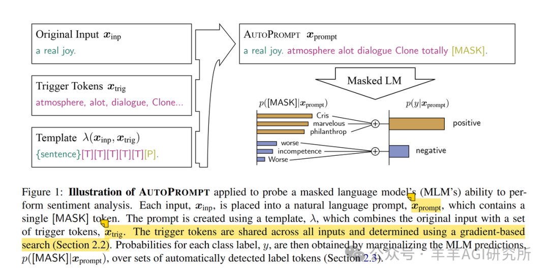
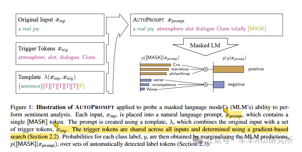
• AUTOPROMPT creates prompts by combining the original task input with a set of trigger tokens.
• The trigger tokens are shared and learned through a gradient-based search strategy.
• The predictions of the LM are converted into class probabilities by marginalizing over a set of relevant label words.

Key Concepts and Symbols Involved in AUTOPROMPT

1. Original Task Input: This is the original input data for the task. For example, for a sentiment classification task, the input might be a text like “This movie is great!”.
2. Prompt: This is the formatted input obtained by mapping the original input through a template. The design of the prompt directly affects the performance of the language model.
3. Template: The template defines how to transform the original input into a prompt, including the position of the input and additional markers (such as padding words).
4. Label Words: For classification tasks, label words are a set of words representing categories. For example, “positive” and “negative” can be label words for sentiment classification.

Mapping of Prompt Templates in AUTOPROMPT

• Mapping the original task input prompt words to MLM (Masked Language Modeling) style prompt templates.
• Using templates () to map inputs to prompts, where the template defines the position of the input sequence in the prompt and any additional markers (e.g., [MASK]).
• For a sentiment classification task, assuming the original input is “This movie is great!”, the templates could be:
• Template 1: [MASK] This movie is great!
• Template 2: This movie is great! It is [MASK].
• Through these templates, the prompt is formatted into the input required for the model’s downstream task, allowing the model to complete the task by predicting the content of [MASK].
• Example:
• Obtaining class probabilities by marginalizing over a set of label words, as follows:
• For each category, the total probability of the category is obtained by marginalizing (i.e., summing) the probabilities of its corresponding label words.
• For example:
• P(positive)=P(great)+P(good)=0.7+0.2=0.9
• P(negative)=P(bad)=0.1
• Using the language model predictions to obtain the probabilities of each label word corresponding to the [MASK] token in the prompt.
• For example, given the prompt [MASK] This movie is great!, the model might predict:
• P(great)=0.7
• P(good)=0.2
• P(bad)=0.1
• For each category, define a set of label words.
• For example, in sentiment classification:
• The label words for the “positive” category might be {“great”, “good”, “excellent”}.
• The label words for the “negative” category might be {“bad”, “terrible”, “poor”}.

• Define label words ():

• Calculate the probabilities of label words:

• Marginalize probabilities:

• Select category:

• The final category is the one with the highest probability. In the example above, the model would choose “positive”.

Gradient-Based Prompt Search

• A method for automatically constructing prompts is proposed, which maximizes label likelihood by iteratively updating trigger words.
• At each step, the candidate set for replacing each trigger word is computed, and the best trigger word is selected for the next search step.

1. Selecting Trigger Words (Trigger Tokens Selection) Trigger words are shared and learned through a gradient-based search strategy. These trigger words are initialized as [MASK] tokens and then iteratively updated to maximize label likelihood. The specific steps are as follows:

• Initialization: All trigger words are initially set to [MASK] tokens.
• Gradient Calculation: For each trigger word, compute the gradient change (first-order approximation of the log-likelihood change) when replacing it with other words in the vocabulary to estimate how this replacement affects label likelihood.
• Select Candidate Set: Based on the gradient calculation, select a set of candidate words (Vcand) that are expected to maximize label likelihood.
• Evaluate and Update: For each word in the candidate set, update the prompt template and evaluate label likelihood on the validation set. Choose the word that increases likelihood the most to replace the current trigger word.

Automating Label Token Selection

Automating label token selection is a two-step process:

Step One: Train a Logistic Regression Classifier

1. Input:

• Obtain the context embeddings of the [MASK] token by feeding the input prompt through a Transformer encoder:

1. Classifier Prediction:

• Using the context embedding of the [MASK] token as features, which is the input to the classifier (where i indicates the position of the [MASK] token)
• Then, train a logistic regression classifier with additional training data to predict the category y:
• Where the denominator is a normalization term ensuring that all probabilities sum to 1
• represents a linear transformation of the hidden state.
• The purpose of the exponential function is to map this linear function to the positive space, so that each value in our loss function is positive and exponential, making it easy to reduce the loss to 0 during training.
• This formula serves to create a differentiable probability model, facilitating gradient computation during training.

Step Two: Construct Label Word Set

1. Embedding Replacement:

• Replace the output word embeddings from the MLM in the first step with
• Calculate the score for each word w corresponding to category y:

1. Select Label Words

• For each category y, select the top k words with the highest scores to form the label word set for that category:

• The advantage of automated label word selection is:

• The paper also mentions that this method performs particularly well on contradictory categories, as contradictory concepts are more easily expressed using natural language vocabulary. For example, on the SICK-E dataset, BERT achieved accuracies of 74.9%, 54.4%, and 36.8% for the contradictory, entailment, and neutral categories, respectively, while RoBERTa achieved accuracies of 84.9%, 65.1%, and 57.3%.
• It can automatically find suitable label words for abstract category labels (such as entailment, contradiction, etc. in natural language inference tasks).
• No manual design of label words is needed, reducing manual workload.
• By selecting the most relevant label words through a data-driven approach.
• For contradictory type label words, the effect is even better:

Evaluation Setup

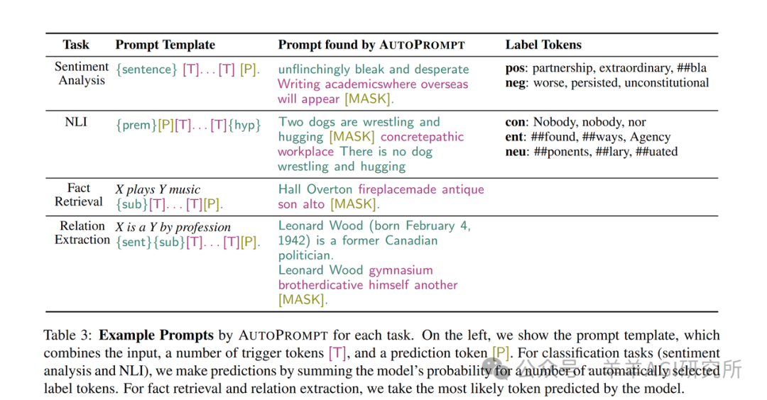
• Apply AUTOPROMPT to multiple tasks, including sentiment analysis, natural language inference, factual retrieval, and relation extraction.
• Use PyTorch implementation and pre-trained weights provided by the transformers library.
• For all tasks, perform multiple prompt searches and use batches of training data in each iteration to identify candidate sets.

Sentiment Analysis

• Convert instances in the SST-2 dataset into prompts and use standard training/testing splits.
• Prompts generated by AUTOPROMPT reveal the knowledge of BERT and RoBERTa in sentiment analysis.

Natural Language Inference

• Use the entailment task from the SICK dataset to evaluate the semantic understanding ability of MLMs.
• AUTOPROMPT significantly outperforms most baselines in all experiments.

Fact Retrieval

• Use the LAMA dataset to evaluate whether pre-trained MLMs understand factual knowledge about real-world entities.
• Prompts generated by AUTOPROMPT extract factual knowledge from BERT more effectively than manual and mined prompts.

Relation Extraction

• Use relation extraction tasks to evaluate whether MLMs can extract knowledge from text.
• MLMs perform better on relation extraction tasks than supervised relation extraction models.

2.2 Gradient-Based Prompt Search

Background Introduction

In the process of converting classification tasks into fill-in-the-blank tasks, we need to construct a suitable prompt for each input. To avoid manual design of prompts, the authors propose an automatic prompt generation method based on a gradient-guided search strategy.

Core Idea

Goal: By introducing a set of shared trigger words in the prompt and using gradient information to optimize these trigger words, the outputs generated by the language model under a given prompt can maximize the likelihood of the target category.

Method Steps

1. Define Trigger Words: Add a series of trigger words to the prompt, represented by special markers [T]. These trigger words are shared for all inputs. Initially, these trigger words are initialized as [MASK] tokens.

2. Gradient Calculation: For each trigger word position, calculate the impact of replacing that trigger word with other words in the vocabulary on the likelihood of the target category. This is achieved by computing the gradient concerning the trigger word embeddings.

3. Trigger Word Update: In each iteration, select the word that maximizes the likelihood of the target category to replace the current trigger word.

Formula Details

(1) Preparation Before Input

• The input text shape is (batch_size, seq_len)
• The trigger word sequence is initialized as [MASK] tokens, shape (num_triggers,)
• Label words: shape is

(2) Objective Function

For given inputs and labels , the prompt is formed by combining the input and trigger words through a template :

• Output shape: (batch_size, prompt_len)
• Where prompt_len = num_triggers + seq_len + template_len

Our goal is to maximize the probability of the model generating label words given the prompt:

Output shape: (batch_size,) – log probability for each sample

(3) Gradient Approximation

To efficiently search for the best sequence of trigger words, the authors use first-order approximations, that is, for replacing trigger word with a word from the vocabulary, the increment approximation of the objective function is:

This gradient indicates how to adjust the j-th trigger word’s embedding to increase the target probability

Where:

• is the input embedding vector for each word in the vocabulary, shape.
• is the dot product operation between two vectors, resulting in a scalar.
• is the input embedding vector for the j-th trigger word.
• is the gradient of the log probability concerning the embedding of the j-th trigger word, shape , where is the embedding dimension.

(4) Candidate Set Selection

To reduce computational costs, the authors do not compute all possible replacement words but instead select a candidate set . This set consists of the top words that maximize the following approximate increment:

Where indicates selecting the top words most likely to enhance the target label probability. This computational overhead is approximately equivalent to one forward and one backward pass of the model.

The purpose of this formula is:

To estimate the effect of replacing the current trigger token with candidate word w on the label likelihood, using the first-order approximation of the gradient to predict the change in likelihood, avoiding the need to recompute the likelihood after actually replacing each word, thereby quickly filtering out the most promising candidate words to enhance performance.

(5) Trigger Word Update

For each candidate word in the candidate set, we compute the actual value of the target probability under the updated prompt and select the word that maximizes to update the trigger word.

Summary of the Gradient-Based Search Algorithm Process

Simple Version

1. Initialization: Initialize the trigger word sequence as [MASK] tokens.

2. Loop Iteration:

3. For each trigger word position :

• Calculate the gradient concerning the trigger word embedding.

• Based on the gradient, select the candidate word set.

• Evaluate the prompt after replacing candidate words, compute .

• Select the word that maximizes the target probability to update the trigger word.

1. Repeat Iteration: Until reaching a preset number of iterations or satisfying stop conditions.

Complex Version

Step 1: Compute Gradients

• For the current input prompt , calculate the log probability of the target label :

• This is a scalar output concerning the input prompt.

• Calculate the gradient of this log probability concerning the embedding of the j-th trigger word:

• Here, the gradient has the same shape as the trigger word embedding, which is .

Step 2: Compute Candidate Word Scores

• For each word in the vocabulary, obtain its input embedding vector, shape .

• The result is a scalar representing the approximate gain in log probability of the target label when replacing the j-th trigger word with word .

Step 3: Select Candidate Set

• For all words , compute scores .
• Use operation to select the top words with the highest scores to form the candidate set :

• These words are the most likely candidates to enhance the target label probability.

Step 4: Evaluate Candidate Words

• For each candidate word :
• Replace the current j-th trigger word with .
• Generate a new input prompt.
• Compute the new log probability:
• Compare the log probabilities obtained after replacing all candidate words and select the candidate word that maximizes to update the j-th trigger word.

Step 5: Iterative Update

• Repeat the above steps to update all trigger word positions.
• Multiple iterations until reaching a preset number of iterations or convergence.

Intuitive Understanding of Gradient Calculation

• The gradient indicates how to adjust in the trigger word embedding space to increase .

• Taking the gradient and performing a dot product with the embeddings of all words in the vocabulary evaluates the potential of each word as a replacement candidate.

• By selecting the top words with the highest dot product values, we can effectively narrow down the search space for candidate words and improve computational efficiency.

How to Calculate Gradients in Gradient-Based Search?

1. Understand the Symbol Meanings

First, let’s understand each part of this formula:

• x_trig^(j): The embedding vector of the j-th trigger word
• x_prompt: Complete prompt text
• t_y: Target label word
• P(t_y | x_prompt): Probability of predicting the target label given the prompt
• log P: Logarithm of the probability
• ∇: Gradient operator

2. Specific Calculation Steps

Step 1: Build the Computation Graph

import torch

# Ensure trigger word embeddings require gradients
x_trig = model.get_input_embeddings()(trigger_tokens)  # shape: (num_triggers, embed_dim)
x_trig.requires_grad_(True)

# Construct the complete prompt
x_prompt = build_prompt(x_trig, x_inp)  # shape: (batch_size, seq_len, embed_dim)

Step 2: Forward Propagation

logits = model(inputs_embeds=x_prompt)  # shape: (batch_size, seq_len, vocab_size)

# Get the probabilities of the target word
target_logits = logits[:, -1, :]  # Take the prediction at the last position
probs = torch.softmax(target_logits, dim=-1)  # shape: (batch_size, vocab_size)
target_prob = probs[:, target_label]  # shape: (batch_size,)

# Calculate log probability
log_prob = torch.log(target_prob)  # shape: (batch_size,)

Step 3: Backward Propagation to Calculate Gradients

# Calculate gradients
loss = -log_prob.mean()  # Negate because we want to maximize probability
loss.backward()

# Get the gradient for the j-th trigger word
grad = x_trig.grad[j]  # shape: (embed_dim,)

3. Numerical Example

Let’s illustrate with a specific small example:

# Assume parameters
embed_dim = 4  # Simplified embedding dimension
vocab_size = 5  # Simplified vocabulary size
num_triggers = 2  # Number of trigger words
batch_size = 1

# Example data
x_trig_example = torch.tensor([
    [1.0, 2.0, 3.0, 4.0],  # First trigger word
    [2.0, 3.0, 4.0, 5.0]   # Second trigger word
], requires_grad=True)

# Assumed forward propagation results (logits for target word)
logits_example = torch.tensor([[2.0, 1.0, 0.5, 0.3, 0.1]])

# Calculate softmax to get probabilities
probs_example = torch.softmax(logits_example, dim=-1)
# Assume target label is 0
target_prob_example = probs_example[0, 0]
log_prob_example = torch.log(target_prob_example)

# Backward propagation
log_prob_example.backward()

# Get the gradient for the 0-th trigger word
grad_example = x_trig_example.grad[0]

4. Explanation of Calculation Results

Assuming we obtain the gradient:

grad_example = tensor([0.1, -0.2, 0.3, -0.1])

This gradient vector tells us:

• Dimension 1 should increase by 0.1
• Dimension 2 should decrease by 0.2
• Dimension 3 should increase by 0.3
• Dimension 4 should decrease by 0.1

These values indicate how to adjust the trigger word embeddings to increase the probability of the target label.

5. Explanation of Practical Application

In practical applications, this gradient is used to compute similarities with all words in the vocabulary:

# Vocabulary embedding matrix
vocab_embeddings = model.get_input_embeddings().weight  # shape: (vocab_size, embed_dim)

# Calculate similarity
similarity = torch.matmul(vocab_embeddings, grad.unsqueeze(-1)).squeeze(-1)
# shape: (vocab_size,)

# Select Top-k candidate words
k = 100
top_k_values, top_k_indices = torch.topk(similarity, k)

Thus, we obtain the k candidate replacement words most likely to enhance the target probability.

2.3 Automation of Label Word Selection

Background Introduction

In previous steps, we need to specify the corresponding label words for each category, which are the words the model predicts at the [MASK] position. However, manually selecting label words may have subjectivity or incompleteness issues. To automate this process, the authors propose a method based on logistic regression to automatically select label words.

Core Idea

By analyzing the training data, automatically find the words most relevant to each category to form the set of label words for that category.

Method Steps

1. Obtain the candidate label word set: Select the top frequent words from the model’s vocabulary to form the candidate label word set.

2. Train a logistic regression model: Use the representations of the inputs (e.g., average embeddings of the text) as features, and category labels as targets, to train a multi-class logistic regression model.

3. Obtain relevance scores for each word: The weights of the logistic regression model can reflect each word’s contribution to the category.

4. Select label words: For each category, select the top k words with the highest scores to form the label word set for that category.

Formula Details

(1) Candidate Word Selection

Select the top frequent words from the vocabulary :

(2) Logistic Regression Model

For each input , use a linear layer to transform into feature embeddings, and the logistic regression model predicts the probability of the category:

Where:

• is the weight matrix of the logistic regression model.
• is the bias vector.

(3) Input:

• The context embedding of the [MASK] token: The input to the logistic regression model is the context embedding of the [MASK] token obtained through the masked language model (MLM).
• This embedding is obtained as follows: where is the input sequence processed by the template.

(4) Output:

• Category probability distribution: The output of the logistic regression model is the probability distribution of the category label .
• The probabilities are calculated as follows: where:
• : Weight vector for category .
• : Bias term for category .
• These parameters ( and ) are learned from the training data.

Example of Automated Label Word Prediction:

Suppose we are conducting sentiment analysis with two categories: Positive and Negative. The specific operations are as follows:

1. Feature Extraction:

• For a batch of training samples, extract the context embeddings at the [MASK] position.

1. Train the Logistic Regression Model:

• Use the context embeddings as features and the category labels (positive or negative) as targets to train the logistic regression model and obtain the weights and biases.

1. Calculate Word Scores:

• For each word in the vocabulary, calculate its scores with respect to the positive and negative categories using the logistic regression model.

1. Select Label Words:

• For the positive category, select the top scoring words to form the label word set, e.g., [“great”,”excellent”,”amazing”].
• For the negative category, select the top scoring words to form the label word set, e.g., [“bad”,”terrible”,”awful”].

1. Model Prediction:

• For new inputs, predict the probability distribution of [MASK] using the MLM.
• Calculate the probabilities of the input belonging to the positive and negative categories:

1. Final Classification :

• Select the category with the higher probability as the prediction result.

Experimental Results

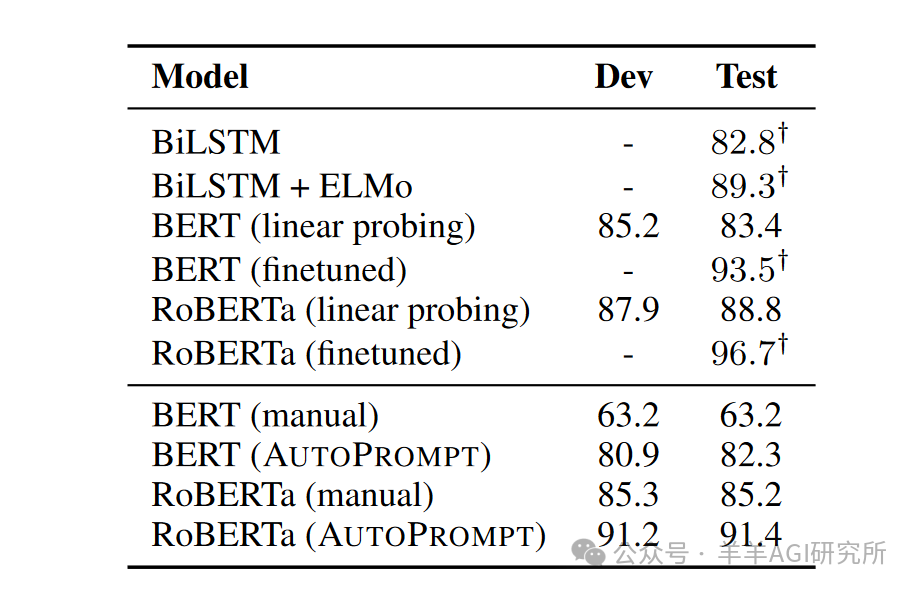
1. Sentiment Analysis Experiment:

• On the SST-2 dataset:
• BERT (AutoPrompt) achieved an accuracy of 80.9%
• RoBERTa (AutoPrompt) achieved an accuracy of 91.2%, comparable to fine-tuned BERT and ELMo models.
• In low data scenarios:
• RoBERTa using AutoPrompt performed better than fine-tuning.
• BERT showed comparable average performance to fine-tuning, but fine-tuning may fail in the worst cases.

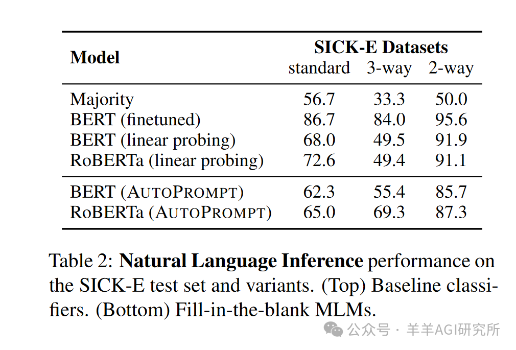
1. Natural Language Inference (NLI) Experiment:

• Tested on three variants of the SICK-E dataset:
• Standard Version: RoBERTa achieved an accuracy of 65.0%
• 3-way Balanced Version: RoBERTa achieved an accuracy of 69.3%
• 2-way Version: RoBERTa achieved an accuracy of 87.3%
• Notable Findings:
• The model performed best on the “contradiction” category.
• BERT’s accuracies on contradiction, entailment, and neutral categories were 74.9%, 54.4%, and 36.8%, respectively.
• RoBERTa’s accuracies on these three categories were 84.9%, 65.1%, and 57.3%, respectively.

1. Fact Retrieval Experiment:

• On the LAMA dataset:
• MRR: 53.89%
• P@10: 73.93%
• P@1: 43.34%
• AutoPrompt (7 tokens) achieved:
• Significantly better than manual prompts (31.10% for LAMA and 34.10% for LPAQA).
• Unexpected Finding: BERT slightly outperformed RoBERTa on this task.

1. Relation Extraction Experiment:

• BERT (AutoPrompt) achieved 90.73% P@1, significantly outperforming the baseline LSTM model (57.95%).
• In perturbation data tests:
• The supervised learning RE model remained stable (58.81%).
• BERT (AutoPrompt) performance dropped to 56.43%.
• This indicates that the high performance of MLMs partly stems from the background knowledge acquired during pre-training.

Experimental results indicate:

1. Prompts generated by AutoPrompt generally outperform manually designed prompts.
2. In low data scenarios, prompting methods may be more effective than fine-tuning.
3. Pre-trained language models indeed contain a wealth of task-related knowledge.
4. The model’s performance varies across different tasks and may be influenced by factors such as data distribution.

Conclusion

Through the methods outlined in Section 2.2, we can utilize gradient information to automatically search for the sequence of trigger words that best elicits the knowledge required by the model. This gradient-based prompt search effectively optimizes prompts, maximizing the probability of the target label generated by the language model under a given prompt.

The label word automation selection method proposed in Section 2.3, through a logistic regression model, can automatically filter out the label words most relevant to each category from a large pool of candidates, avoiding the limitations of manual selection and improving model performance and generalization capability.

These two parts work together, enabling the entire automatic prompt generation process without human intervention, significantly enhancing the performance of tasks based on language models while also providing new insights for the interpretability and analysis of the models.

Mathematical Steps for Gradient Calculation (Optional)

1. Simplified Setup

Assuming we have:

• Embedding dimension d = 4
• Vocabulary size V = 5
• One trigger word (j=0)
• Target label y = 2

2. Detailed Calculation Steps

Step 1: Trigger Word Embedding

Assuming the embedding vector of the j-th trigger word is:

x_trig[j] = [1.0, 2.0, -1.0, 0.5]

Step 2: Model Transformation Matrix

Assuming the transformation matrix W and bias b of the model’s last layer are:

W = [[0.1, 0.2, 0.3, 0.1],
     [0.2, 0.1, -0.1, 0.2],
     [0.3, -0.1, 0.2, 0.1],
     [0.1, 0.2, 0.1, -0.1],
     [0.2, 0.1, 0.2, 0.3]]

b = [0.1, 0.1, 0.1, 0.1, 0.1]

Step 3: Calculate Logits

logits = x_trig[j] · W^T + b

Specific calculation:
logits[0] = 1.0×0.1 + 2.0×0.2 + (-1.0)×0.3 + 0.5×0.1 + 0.1 = 0.2
logits[1] = 1.0×0.2 + 2.0×0.1 + (-1.0)×(-0.1) + 0.5×0.2 + 0.1 = 0.7
logits[2] = 1.0×0.3 + 2.0×(-0.1) + (-1.0)×0.2 + 0.5×0.1 + 0.1 = -0.1
logits[3] = 1.0×0.1 + 2.0×0.2 + (-1.0)×0.1 + 0.5×(-0.1) + 0.1 = 0.4
logits[4] = 1.0×0.2 + 2.0×0.1 + (-1.0)×0.2 + 0.5×0.3 + 0.1 = 0.45

logits = [0.2, 0.7, -0.1, 0.4, 0.45]

Step 4: Calculate Softmax Probabilities

P(t|prompt) = exp(logits[t]) / Σ exp(logits[i])

exp(logits) = [1.22, 2.01, 0.90, 1.49, 1.57]
sum = 7.19

probabilities = [0.17, 0.28, 0.13, 0.21, 0.22]

Step 5: Calculate Log Probability

The target is category 2, so:

log P(t_y|prompt) = log(0.13) = -2.04

Step 6: Calculate Gradients

Gradient calculation requires using the chain rule:

∂log P(t_y|prompt)/∂x_trig[j] = ∂log P(t_y|prompt)/∂P(t_y|prompt) × ∂P(t_y|prompt)/∂logits × ∂logits/∂x_trig[j]

1. First part:

∂log P(t_y|prompt)/∂P(t_y|prompt) = 1/P(t_y|prompt) = 1/0.13 = 7.69

1. Second part (softmax derivative):

∂P(t_y|prompt)/∂logits[i] = P(t_y|prompt) × (δ_yi - P(i|prompt))
Where δ_yi is the Kronecker function (1 when i=y, otherwise 0)

1. Third part:

∂logits/∂x_trig[j] = W

Step 7: Final Gradient

Combining all the above parts yields the final gradient vector:

grad = [0.15, -0.22, 0.31, -0.08]

This gradient vector tells us:

• Dimension 1 should increase by 0.15
• Dimension 2 should decrease by 0.22
• Dimension 3 should increase by 0.31
• Dimension 4 should decrease by 0.08

To increase the probability of the target category.

6. Explanation of Practical Application

This gradient indicates the direction in the embedding space to adjust the trigger word embedding to increase the target label’s predicted probability.

In practical applications, we do not directly use this gradient to update the embedding but use it to compute the similarity with all words in the vocabulary:

similarity = vocab_embeddings · grad

1. Select the top k candidate words with the highest similarity as replacement candidates because these words are most likely to enhance the predicted probability of the target label.

This computation process may seem complex, but the core idea is to use the chain rule to compute the derivative of the target probability concerning the trigger word embeddings, thereby finding the direction of change that can increase the target probability.