Introduction to Deep Learning

Deep learning (Deep Learning) algorithms are currently a highly regarded category of algorithms in the industry. In fact, whenever deep learning is mentioned at technical sharing events or conferences, it immediately attracts widespread attention.

Now, let’s introduce some concepts of deep learning. First, what new changes have emerged in our lives with the development of deep learning? Recently popular technologies, such as AlphaGo and Alibaba Cloud’s ET robot, are actually outcomes of deep learning algorithms in the field of artificial intelligence. Through various media, we can learn that many robots possess the ability to converse and recognize faces. Artificial intelligence gives people the impression that it can simulate human thought processes through machine algorithms, which is also the reason for the birth of artificial neural network algorithms, as deep learning algorithms are derived from artificial neural network algorithms.

Deep learning algorithms originated from humanity’s imitation of brain neurons. In 1958, David Hubel and Torsten Wiesel from Johns Hopkins University conducted an experiment where they connected electrodes to the brain neurons of a cat to measure the relationship between the cat’s vision and its neurons. They displayed various shapes in front of the cat to see if a specific area in the brain would respond to certain features. Ultimately, they discovered a type of neuron cell called direction-sensitive neurons, which only activated when an object’s edge pointed in a certain direction. This experiment revealed some physiological laws, showing that when organisms recognize certain individuals, the brain internally performs multiple layers of abstraction, breaking down each thing into particles through neurons and then responding based on the understanding of these particles. When we see faces, the brain has already abstracted each face into small particles (see Figure 1).

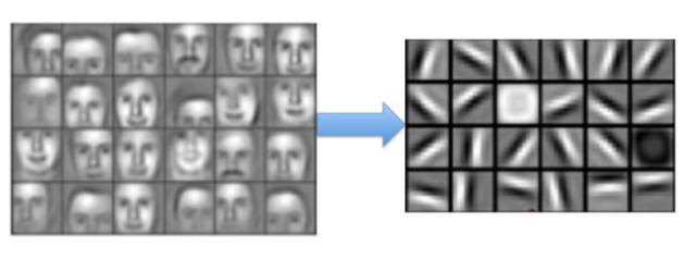
Figure 1: Brain Abstraction

Research has found that this abstraction process is not achieved overnight but is accomplished through layer-by-layer abstraction by neurons, forming a fundamental architecture for neural networks. Deep learning inherits this architecture, as shown in Figure 2.

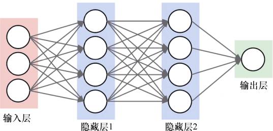
Figure 2: Neural Network Architecture

Data flows into the entire algorithm architecture through the input layer. For example, if the input data is a picture of a face, then in hidden layer 1 and hidden layer 2 (the number of hidden layers can be many, but only two layers are drawn here), the face is abstracted into particles, with each neuron in the hidden layers judging certain feature information of the input data, ultimately outputting the judgment result. Based on this biomimetic brain neuron architecture, artificial neural networks were born, and deep learning algorithms inherited this architecture, eventually leading to a transformative algorithmic change made by the machine learning pioneer Hinton, pushing deep learning to new heights. In 2006, Hinton published a paper on deep learning titled “A Fast Learning Algorithm for Deep Belief Nets,” which truly sparked a wave of interest in deep learning in academia and industry. Deep learning quickly saw disruptive developments in the learning and understanding of speech, images, and text.

Deep learning is ultimately a type of machine learning. If we classify machine learning, besides categorizing it into supervised learning, unsupervised learning, semi-supervised learning, and reinforcement learning, it can also be divided into shallow learning algorithms and deep learning algorithms based on the depth of the algorithm’s network.

1. Shallow Learning Algorithms

Shallow learning (Shallow Learning), as the name suggests, refers to neural networks with fewer hidden layers. Algorithms such as Support Vector Machine (SVM) and Logistic Regression (LR) can be considered shallow learning, also known as conventional machine learning algorithms, because these learning methods do not involve the multi-level abstraction of features, making their architecture simpler compared to deep learning. Taking logistic regression as an example, it simply inputs data into the Sigmoid formula and utilizes gradient descent or other methods to calculate the gradient based on the difference between the result and the predicted value, continuously reducing the gradient until the regression coefficients converge. The shallow learning mentioned now is all supervised learning. The core idea of supervised learning is to optimize the cost function. In shallow algorithm calculations, by solving the gradient, the direction for optimizing the function is found. However, this idea is limited to shallow machine learning algorithms because, in shallow algorithms, there are fewer layers, making it easy to propagate the influence of the target column forward by calculating the gradient. However, in deep learning algorithms, due to the many hidden layers, each layer can be understood as a functional form. When solving for the partial derivative coefficients of each layer, the variables of multi-layer composite functions must be considered, so applying the traditional shallow algorithm’s ideas to train multi-level deep learning networks may not yield ideal results.

Another difference between shallow algorithms and deep learning algorithms lies in how features are handled. Shallow algorithms require manual feature abstraction or derivation when dealing with certain classification scenarios, and the quality of these features not only tests the engineer’s business experience but also significantly impacts model training. This structured data of shopping behavior is shown in Table 1.

Table 1: Shopping Behavior Data

For the structured data shown in Table 1, the features can be easily abstracted. However, for images or audio files, the features of such data may be very complex, making it very difficult to construct features solely based on manual rules. This complexity in feature handling is also a distinction between shallow machine learning and deep learning.

Having introduced shallow learning, it is evident that there are differences between shallow learning and deep learning in terms of model tuning ideas and feature handling. Currently, with the development of statistical theory and computational capabilities, algorithms like logistic regression and support vector machines have been widely applied, especially in recommendation systems or certain classification scenarios. In environments where feature handling is not complex, shallow learning often achieves good results. However, for data with complex feature environments, such as images, audio, and text, deep learning algorithms may need to play a more significant role.

2. Deep Learning Algorithms

Deep learning, as the name implies, emphasizes the characteristic of being “deep.” The structure of the algorithm shows that deep learning inherits the characteristics of neural networks and is composed of multiple layers. In Figure 3, each circle mimics brain neurons, represented mathematically as computational nodes.

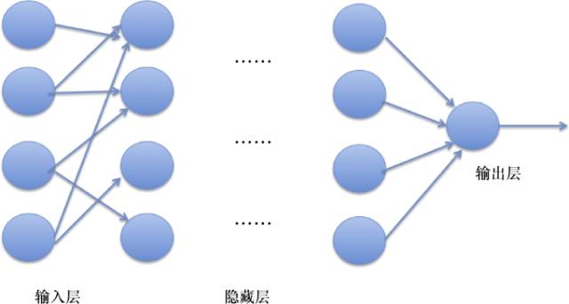
Figure 3: Deep Learning Network

Deep learning consists of three parts: input layer, hidden layers, and output layer. The hidden layers can contain many layers, such as 7 layers, 8 layers, or even more. Compared to shallow learning, deep learning is evidently more complex in terms of computational layers. Because deep learning has many hidden layers, simply using the shallow algorithm’s model optimization idea to optimize each layer’s parameters can adversely affect model accuracy. Hence, in model training, deep learning adopts a different idea—the backpropagation algorithm.

The backpropagation algorithm, also known as the BP algorithm (backpropagation algorithm), is a type of supervised learning algorithm. The core idea of the BP algorithm is the chain rule of derivatives. The BP algorithm is commonly used to solve optimization problems in neural networks. The difference from the optimization solving of shallow algorithms is that the BP algorithm can use the chain rule to iteratively calculate the gradient for each layer. Chain computation can be understood as when optimizing the model using the BP algorithm, the entire chain of partial derivatives from back to front is considered when solving the gradient, and then each layer’s weights are updated. Although the BP algorithm is a simple and efficient optimization algorithm in deep learning, if applied to multi-layer deep learning, the influence of the target column on each preceding layer is certainly diminishing layer by layer. As shown in Figure 4, if the final target column’s influence on each layer is abstracted into a numerical value, then in the algorithm model, if many hidden layers exist, the BP algorithm’s target value’s influence on the earlier hidden layers will certainly diminish layer by layer. This decay can cause significant inaccuracies in the model. Therefore, in the optimization process of deep learning models, many auxiliary means are often needed to optimize the BP algorithm.

Figure 4: BP Algorithm Propagation

Next, let’s briefly introduce the idea of optimization. The training process of deep learning models is bidirectional, with the input to output as the first chain and output to input as the second chain (see Figure 5).

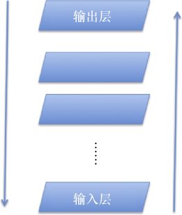
Figure 5: Two Chains of Deep Learning

First, let’s talk about the first chain. Deep learning is trained bottom-up, where each time only one layer of the network is trained, and the training result serves as the input for the next layer. This process resembles a model system continuously refining the data abstraction. For instance, if the input data is a picture of a cat’s head, the first layer may abstract some pixels of the cat, then some lines in the subsequent hidden layers, and finally gradually abstract the outline of the cat. The overall effectiveness of the final model is to recognize whether the input data describes a cat. The second chain, which is top-down, mainly utilizes backpropagation to fine-tune the parameters of each layer because having more than 5 hidden layers in deep learning significantly impacts the results. Both chains involve many mathematical optimization methods.

In fact, the layer-by-layer training of the model discussed earlier is the process of deep learning continuously abstracting features. Another significant difference between deep learning and shallow learning lies in how features are handled. In shallow learning, features are generated through manual processing and extraction, which has poor extensibility for complex feature scenarios like graphical data. Deep learning can automatically construct features through algorithms, mapping features to different dimensional spaces. Next, let’s introduce the autoencoder algorithm that abstracts features layer by layer.

The core idea of the autoencoder (AutoEncoder) is to generate a function F through training such that F(x) is approximately equal to x, meaning to obtain a function that makes the input and output as similar as possible. What is the significance of doing this? Let’s first observe Figure 6.

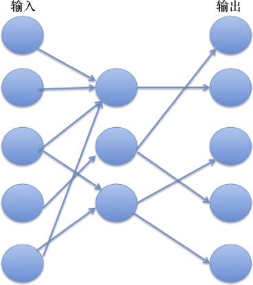
Figure 6: Autoencoder

As shown in Figure 6, each circle represents a neuron. If the input is data from 5 neurons x, the output data through the transformation of 3 neurons is F(x). If F(x) ≈ x, it means that the 3-dimensional data can reconstruct the 5-dimensional input data, and the reconstructed data is almost identical to the original data. In this process, information compression occurs, meaning that the correlation between input data can be utilized through automatic feature extraction, using low-dimensional features to restore high-dimensional data. If applied to image model recognition, it is akin to finding a method to reconstruct an image through points, edges, and lines, with these points, edges, and lines being features mined through the autoencoder.

This is a brief introduction to the model training and feature extraction of deep learning. Overall, deep learning performs well in scenarios with very complex features, such as image recognition, voice recognition, and text analysis.

3. Summary of Differences

Previously, shallow learning and deep learning were introduced separately. Compared to shallow machine learning algorithms, deep learning has a deeper architectural layer and significantly greater computational complexity.

• Target Scene. Currently, shallow learning remains the mainstream application of machine learning, mainly used to solve data analysis for log-type data, especially for predictions of structured numerical data. Deep learning primarily addresses complex feature scenarios, such as image recognition, text analysis, and voice recognition. With the development of open-source frameworks for deep learning and computational resources, more and more business scenarios are attempting to solve problems through deep learning. This is also the reason why some international internet giants have established research institutions to invest heavily in deep learning.

• Feature Abstraction. In terms of feature handling, shallow learning mainly constructs features manually, requiring extensive business background knowledge, and the extensibility of this manual feature extraction method is not particularly good. Deep learning adopts an autoencoder approach, abstracting features layer by layer, which works well for complex feature extraction scenarios.

• Model Training. In model training, shallow learning, due to its fewer architectural layers, can be trained and optimized using supervised methods through single-layer gradient descent. In deep learning, model training often requires two chains—from front to back and from back to front—to optimize the model, and during the training process, the partial derivative relationships of functions between different layers must be considered.

These are some introductions and analyses of the differences between deep learning and shallow learning.

Readers who understand deep learning must have frequently heard of several commonly used structures: DNN, CNN, and RNN. There are many types of deep learning structures, but these three are the most frequently encountered. In fact, these three structural models are not parallel; DNN refers to a general term for algorithms with deep learning networks, CNN is primarily a spatial concept deep learning structure, and RNN is a temporal concept deep learning structure. Next, let’s introduce these three deep learning models separately.

Deep Neural Network (DNN) specifically refers to neural networks with a deep structure, as shown in Figure 7.

Figure 7: DNN Structure

DNN was created by the master of deep learning, Geoff Hinton, and has been applied in various scenarios. DNN generally refers to multi-layer neural networks, where the hidden layers are interconnected. Different structures, such as CNN and RNN introduced later, are derived based on the type and characteristics of the data being processed.

Convolutional Neural Network (CNN) is a special type of deep learning structure, mainly used to address complex spatial feature problems through convolution. What is a spatial problem? A typical example is the image recognition problem. Many models we encounter for license plate recognition and facial recognition rely on CNN for training. The reason CNN performs well on image data is that image features are very complex. Since algorithms can only process standardized data, image data must undergo binary conversion before entering the algorithm model for training. The specific transformation effect is shown in Figure 8 (the image is sourced from “A Beginner’s Guide To Understanding Convolutional Neural Networks”), where a photo of a running dog is converted into numerical data.

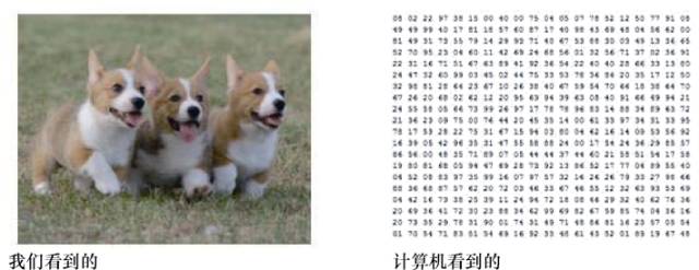
Figure 8: Image Transformation

In the process of converting non-structured data, image data is transformed into matrix-like binary data based on pixels and size. For example, an image is converted into a 32×32×3 array, where 32×32 represents the image’s pixels (interpreted as the image’s length multiplied by its height), and multiplying by 3 represents the RGB (color) values. Based on this data form, if feature training is conducted for each pixel point, the parameters that each hidden layer needs to train will be extremely large. If the parameters for each hidden layer are overly complex, it can easily lead to local overfitting issues. To address this issue of training numerous feature parameters, CNN utilizes convolution kernels as intermediaries for weight propagation, significantly reducing the computational complexity of each layer.

Next, let’s introduce the CNN model architecture using a description image of LCNN LeNet-5 (see Figure 9). LeNet-5 is an open-source CNN model organization, accessible at http://yann.lecun.com/exdb/lenet/.

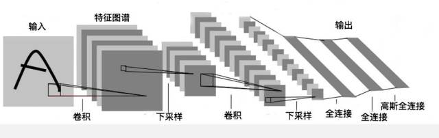
Figure 9: CNN Architecture

Figure 9 illustrates the architecture for handwritten digit recognition achieved through CNN. It can be seen that the CNN architecture includes several key elements: convolutions, subsampling, and full connection, which will be introduced separately below.

(1) Convolutions. First, let’s introduce the principle of convolution kernels, as shown in Figure 10, where the small square marked with a dashed line represents a convolution kernel.

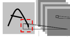
Figure 10: Convolution Kernel Example

A convolution kernel can be understood as a small square that is smaller than the image size. For instance, if the image of the letter “A” is sized 5×5×3, the convolution kernel can be a 3×3×3 small square, which scans the input data matrix.

Next, let’s illustrate how the convolution kernel scans an image through an example. Suppose the input image, disregarding RGB, is a 5×5 matrix data as follows.

3 5 2 6 8

2 4 5 9 6

5 7 8 4 1

3 6 2 7 3

3 7 5 6 8

Now let’s see what happens when this data is processed by the convolution kernel. Suppose the convolution kernel is a 3×3 square, represented as follows.

−3 2 1

2 −5 3

4 5 −2

During convolution calculations, the convolution kernel needs to scan the input data. Here, we will introduce the convolution calculation principle using a portion of the scanning process (see Figure 11).

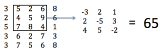
Figure 11: Scanning Principle

When scanning the part of the input matrix circled in black, the following calculation is performed.

−3×5 + 2×2 + 1×6 + 2×4 − 5×5 + 3×9 + 4×7 + 5×8 − 2×4 = 65

After scanning the matrix, the input changes from a 5×5 matrix to a 3×3 matrix, achieving parameter compression. Each layer processes the image through a convolution kernel, simplifying the complex parameter training process, allowing the convolution kernel to learn the feature descriptions of the input data. The entire CNN learning process determines the specific values of the convolution kernels.

(2) Subsampling. When observing the CNN architecture of LeNet-5 (see Figure 9), it can be noted that in addition to the convolution layers mentioned above, there are also subsampling layers interspersed. The role of the subsampling layer is to perform self-sampling on the image, reducing the amount of data processed while retaining as much effective information as possible. The subsampling layer is also represented in deep learning as a pooling layer. There are various pooling methods; here we will introduce a relatively simple method—max pooling (Maxpooling). The principle of max pooling is to select the maximum value from each small area as the output.

To illustrate max pooling, consider the input data structured as 4×4, which can be divided into 4 small squares of 2×2. Max pooling takes the largest value from each part as the output, which preserves the main features of the data while reducing computational complexity.

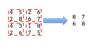
Figure 12: Max Pooling Example

(3) Full Connection. Through the CNN architecture (see Figure 9), we learn that after experiencing two rounds of convolution and sampling processes, numerous feature maps are generated. These feature maps can be viewed as representations of the input image’s positional information and expressions. Different feature maps represent different contents, such as the position of a certain point or the orientation of a certain module in a letter. However, the task at hand is to recognize the letter