Abstract: Training deep models has been a long-standing challenge. In recent years, a series of methods represented by hierarchical and layer-wise initialization have brought hope to training deep models and have achieved success in various application fields. The parallelization framework and training acceleration methods for deep models are important cornerstones for deep learning to become practical…
Training deep models has been a long-standing challenge. In recent years, a series of methods represented by hierarchical and layer-wise initialization have brought hope to training deep models and have achieved success in various application fields. The parallelization framework and training acceleration methods for deep models are important cornerstones for deep learning to become practical, with multiple open-source implementations available for different deep models. Companies such as Google, Facebook, Baidu, and Tencent have also implemented their own parallelization frameworks. Deep learning is currently the most intelligent learning method closest to the human brain, and this revolution ignited by deep learning has brought artificial intelligence to a new level, profoundly impacting a large number of products and services.
1. The Revolution of Deep Learning
Artificial Intelligence (AI) attempts to understand the essence of intelligence and create intelligent machines that can respond similarly to human intelligence. If machines are extensions of the human hand and vehicles are extensions of the human leg, then artificial intelligence is an extension of the human brain, and can even help humans evolve and surpass themselves. AI is also one of the most cutting-edge and mysterious disciplines in computer science, where scientists hope to create intelligent machines that can replace human thinking, and artists have written this theme into novels and films, provoking endless imagination. However, as a serious discipline, AI has not developed smoothly over the past half century. Many past efforts were still based on rapid search and inference of certain preset rules, which is far from true intelligence, or in other words, far from creating machines with abstract learning capabilities like humans.
In recent years, deep learning has directly attempted to solve the problems of abstract cognition and has made groundbreaking progress. The revolution ignited by deep learning has brought artificial intelligence to a new level, with significant academic meaning and strong practicality, leading to large-scale investments from the industrial sector, benefiting a large number of products.
In 2006, machine learning pioneer and University of Toronto professor Geoffrey Hinton published an article in Science [1] proposing that deep belief networks (DBN) could use unsupervised layer-wise greedy training algorithms, bringing hope to training deep neural networks.
In 2012, Hinton led his students to achieve astonishing results on the largest image database, ImageNet [2], reducing the Top-5 error rate from 26% to 15%.
In 2012, a dream team led by top AI and machine learning scholars Andrew Ng and distributed systems expert Jeff Dean began building the Google Brain project, using a parallel computing platform with 16,000 CPU cores to train deep neural networks with over 1 billion neurons, achieving groundbreaking results in speech recognition and image recognition [3]. The system analyzed selected videos from YouTube and trained deep neural networks in an unsupervised manner, automatically clustering images. When “cat” was input into the system, it identified cat faces without external interference.
In 2012, Microsoft Chief Research Officer Rick Rashid demonstrated an automatic simultaneous interpretation system [4] at the 21st Century Computing Conference, which converted his English speech in real-time into a Chinese speech that closely matched his tone and pronunciation. Simultaneous interpretation requires passing through three steps: speech recognition, machine translation, and speech synthesis. The system performed smoothly and received unanimous recognition, with deep learning being the key technology in this system.
In 2013, Google acquired a neural network startup called DNN Research, which had only three people: Geoffrey Hinton and his two students. This acquisition did not involve any products or services; it was simply hoped that Hinton could build deep learning as a core technology supporting Google’s future. In the same year, New York University professor and deep learning expert Yann LeCun joined Facebook as the director of the artificial intelligence lab [5], responsible for deep learning research, exploring the massive information contained in user images and hoping to provide users with a more intelligent product experience in the future.
In 2013, Baidu established the Baidu Research Institute and the subordinate Institute of Deep Learning (IDL), applying deep learning to speech recognition, image recognition, retrieval, and advertising CTR prediction (Click-Through-Rate Prediction, pCTR), achieving internationally leading levels in image retrieval. In 2014, they brought Andrew Ng on board, who is the director of the Stanford AI Lab and was selected as one of Time magazine’s 100 most influential people in the world, representing the tech industry.
If Hinton’s 2006 paper published in Science [1] only sparked a research boom in deep learning in academia, then the recent competition among major companies to recruit top talent from academia to industry marks the true practical phase of deep learning, which will have a profound impact on a series of products and services, becoming the powerful technological engine behind them.
Currently, deep learning has achieved groundbreaking progress in several major areas: in speech recognition, deep learning has replaced the Gaussian Mixture Model (GMM) in acoustic models with deep models, achieving about a 30% reduction in error rates; in image recognition, by constructing deep convolutional neural networks (CNN) [2], the Top-5 error rate was significantly reduced from 26% to 15%, and further reduced to 11% by deepening the network structure; in natural language processing, deep learning has achieved results comparable to other methods, but can eliminate the tedious feature extraction steps. It can be said that so far, deep learning is the most intelligent learning method closest to the human brain.
2. Basic Structure of Deep Models
The model used in deep learning is the Deep Neural Networks (DNN) model, which consists of multiple hidden layers (Hidden Layer). Deep learning utilizes the hidden layers in the model to transform the original input into shallow features, medium features, high-level features, and ultimately to the final task objective, through feature combinations.
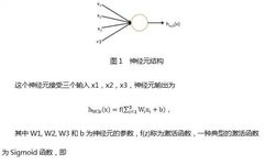
Deep learning originated from the study of artificial neural networks. Let’s review artificial neural networks. A neuron is shown in the figure below [6]:
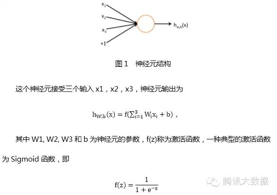
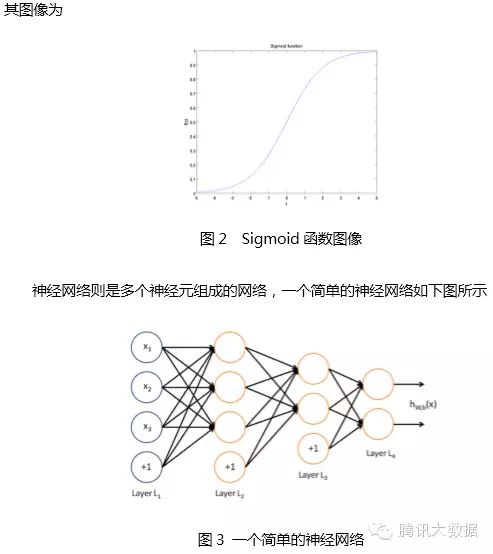
The circles represent the input of the neural network, and the circle marked with “+1” is called the bias node, which is the intercept term. The leftmost layer of the neural network is called the input layer (in this case, there are 3 input units, excluding the bias unit); the rightmost layer is called the output layer (in this case, the output layer has 2 nodes); the middle nodes are called hidden layers (in this case, there are 2 hidden layers, with 3 and 2 neurons respectively, excluding the bias unit), as their values cannot be observed in the training sample set. Each connection in the neural network corresponds to a connection parameter, and the number of connections corresponds to the number of parameters in the network (in this example, there are a total of 4×3 + 4×2 + 3×2 = 26 parameters). Solving this neural network requires a sample set of (x(i), y(i)), where x(i) is a 3-dimensional vector and y(i) is a 2-dimensional vector.
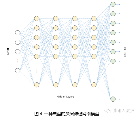
The above figure is a shallow neural network, while the figure below is a deep neural network used for speech recognition, which has 1 input layer, 4 hidden layers, and 1 output layer, with all neurons in adjacent layers fully connected.
3. Reasons for Choosing Deep Models
Why construct a deep network structure with so many hidden layers? There are some theoretical bases behind it:
3.1 Naturally Hierarchical Features
For many training tasks, features have a natural hierarchical structure. Taking speech, images, and text as examples, the hierarchical structure is roughly shown in the table below.
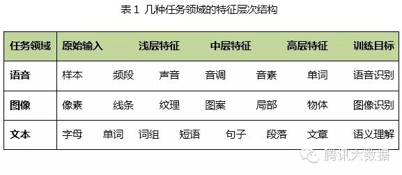
Taking image recognition as an example, the original input of the image is pixels, adjacent pixels form lines, multiple lines form textures, which further form patterns, and patterns constitute the local appearance of objects, leading to the entire shape of the object. It is not difficult to see that there is a connection between the original input and shallow features, and through medium features, step by step, the connection to high-level features can be obtained. It would undoubtedly be difficult to jump directly from the original input to high-level features.
3.2 Bionic Basis
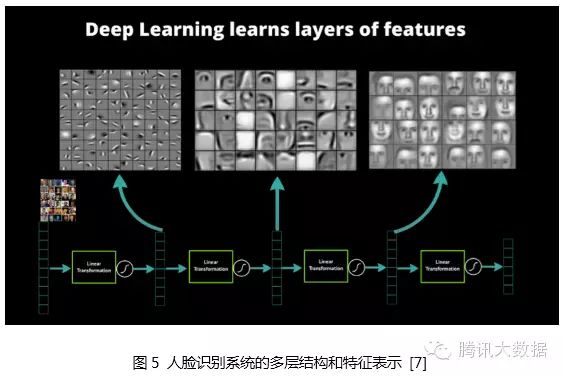
Artificial neural networks themselves simulate the human nervous system, and this simulation has a bionic basis. In 1981, David Hubel and Torsten Wiesel discovered that the visual cortex is hierarchical [8]. The human visual system contains different visual neurons, and these neurons have a corresponding relationship with the stimuli received by the pupil (system input) (the connection parameters between neurons); that is, after receiving a certain stimulus (for a given input), some neurons become active (are activated). This confirms that the work of the human nervous system and brain is actually a continuous process of transmitting low-level abstractions to high-level abstractions, where high-level features are combinations of low-level features, and the higher the level of features, the more abstract they become.
3.3 Hierarchical Representability of Features
The hierarchical representability of features has also been confirmed. Around 1995, Bruno Olshausen and David Field [9] collected many black-and-white landscape photos and found 400 basic fragments of 16×16 from these photos, and then found other fragments of the same size from the photos, hoping to express other fragments as linear combinations of these 400 basic fragments while minimizing the error and using as few fragments as possible. After representation, by fixing other fragments, they selected more suitable combinations of basic fragments to optimize the approximation results. After repeated iterations, they obtained the best combinations of basic fragments that could represent other fragments. They found that these basic fragment combinations were the edge lines of different objects in different orientations.
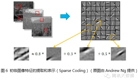
This indicates that effective feature extraction can abstract pixels into higher-level features. Similar results also apply to speech features.
4. From Shallow Models to Deep Models
The previous section discussed the structure of deep models and their advantages. In fact, deep models have powerful expressive capabilities and can effectively extract high-level features like humans, which is not a new discovery. So why have deep models only gained widespread attention and application in recent years? Let’s start with traditional machine learning methods and shallow learning.
4.1 Shallow Models and Training Methods
The backpropagation algorithm (BP algorithm) [10] is a gradient computation method for neural networks. The backpropagation algorithm first defines the cost function of the model on the training samples, and then calculates the gradient of the cost function for each parameter. The backpropagation algorithm cleverly utilizes the rule that the gradient of lower-layer neurons can be derived from the residuals of upper-layer neurons, and the solving process is just as the name of the algorithm suggests, calculating in reverse layer by layer from top to bottom until all parameter gradients are obtained. The backpropagation algorithm can help train statistical machine learning models, mining statistical patterns from a large number of training samples, and can then predict unlabelled data. This statistical-based learning method has many advantages over traditional rule-based methods [11].
In the 1980s and 1990s, a series of machine learning models were proposed, the most widely used being Support Vector Machines (SVM) [12] and Logistic Regression (LR) [13], which can be seen as shallow models containing one hidden layer and no hidden layer, respectively. During training, the backpropagation algorithm can be used to calculate gradients and then use the gradient descent method to find the optimal solution in the parameter space. Shallow models often have convex cost functions, making theoretical analysis relatively simple, and the training methods easy to master, leading to many successful applications.
4.2 Training Difficulty of Deep Models
The limitations of shallow models lie in their limited parameters and computational units, which restrict their ability to represent complex functions, and their generalization ability is limited for complex classification problems. Deep models can precisely overcome this weakness of shallow models, but training deep models using backpropagation and gradient descent faces several prominent issues [14]:
1. Local Optima. Unlike shallow models’ cost functions, each neuron in deep models undergoes nonlinear transformations, making the cost function a highly non-convex function, and using gradient descent can easily lead to local optima.
2. Gradient Vanishing. When propagating gradients using the backpropagation algorithm, as the propagation depth increases, the magnitude of the gradient can decrease sharply, leading to very slow weight updates for shallow neurons, preventing effective learning. As a result, the deep model may become a shallow model where only the last few layers can be modified.
3. Data Acquisition. Deep models have strong expressive power, and the number of parameters in the model also increases accordingly. A small training dataset cannot train a model with so many parameters; massive labeled data is needed, or it will lead to severe overfitting.
4.3 Training Methods for Deep Models
Despite the significant challenges, Professor Hinton did not give up. He has been engaged in related research for 30 years and finally made groundbreaking progress. In 2006, he published an article in Science [1], igniting a wave of deep learning in academia and industry. The two main points of this article are:
1. Multi-hidden-layer artificial neural networks have excellent feature learning capabilities, and the features learned provide a more essential characterization of the data, which is beneficial for visualization or classification.
2. The difficulty of training deep neural networks can be effectively overcome through “layer-wise pre-training”; the article provides an unsupervised layer-wise pre-training method.
The excellent feature characterization ability has been mentioned earlier, so it will not be repeated here. The next focus will be on explaining the “layer-wise initialization” method.
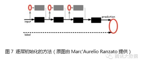
Given the original input, the first layer of the model must be trained first, which is the black box on the left side of the figure. The black box can be seen as an encoder that encodes the original input into the primary features of the first layer, and this encoder can be viewed as a kind of “cognition” of the model. To verify that these features are indeed an abstract representation of the input and that not too much information is lost, a corresponding decoder must be introduced, which is the gray box on the left side of the figure, and can be seen as the model’s “generation”. To ensure that cognition and generation are consistent, the original input must be encoded and then decoded to roughly restore the original input. Therefore, the error between the original input and the input after encoding and decoding is defined as the cost function, while training both the encoder and decoder. Once training converges, the encoder becomes the first layer model we want, and the decoder is no longer needed. At this point, we have obtained the first layer abstraction of the original data. Fixing the first layer model, the original input is mapped to the first layer abstraction, which is treated as input to continue training the second layer model, and then train the third layer model based on the first two layers, and so on, until the highest layer model is trained.
After layer-wise initialization is completed, labeled data can be used to conduct overall supervised training of the model using the backpropagation algorithm. This step can be seen as fine-tuning the entire multi-layer model. Since deep models have many local optimal solutions, the initialization position of the model will largely determine the quality of the final model. The “layer-wise initialization” step is designed to place the model at a position closer to the global optimum, thereby achieving better results.
4.4 Comparison of Shallow Models and Deep Models
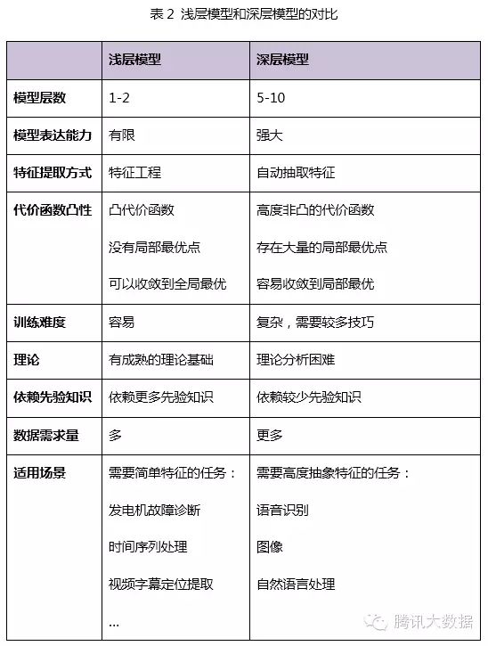
Shallow models have an important characteristic: they rely on human experience to extract sample features, and the model’s input consists of these pre-selected features, with the model only responsible for classification and prediction. In shallow models, the most important factor is often not the quality of the model, but the quality of feature selection. Therefore, most human effort is invested in feature development and screening, which not only requires a deep understanding of the task domain but also consumes a lot of time in repeated experiments and explorations, which limits the effectiveness of shallow models.
In fact, layer-wise initialization of deep models can also be seen as a process of feature learning, where the hidden layers abstractly represent the original input step by step, learning the data structure of the original input and finding more useful features, thereby ultimately improving the accuracy of classification problems. Once effective features are obtained, the overall training of the model can proceed smoothly.
5. Hierarchical Components of Deep Models
Deep models consist of multiple hidden layers. What is the specific structure of each layer? This section introduces some common basic layer components of deep models.
5.1 Auto-Encoder
A common deep model is constructed using auto-encoders [6]. Auto-encoders can utilize a set of unlabeled training data {x(1), x(2), … } (where x(i) is an n-dimensional vector) for unsupervised model training. It uses the backpropagation algorithm to bring the target value close to the input value. The following is an example of an auto-encoder:
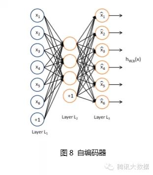
Auto-encoders attempt to train an identity function, making the output close to the input value. The identity function seems to have no learning significance, but considering that the number of hidden neurons (3 in this example) is less than the dimensionality of the input vector (6-dimensional in this example), the hidden layer effectively becomes a compressed representation of the input data, or an abstract simplified representation. If the network’s input is completely random, compressing a high-dimensional vector into a low-dimensional vector would be challenging. However, training data often contains specific structures, and auto-encoders will learn the correlations of these data, thus obtaining effective compressed representations. After actual training, if the cost function is smaller, it indicates that the input and output are closer, suggesting that this encoder is more reliable. Of course, after training the auto-encoder, only the encoder part is needed for actual use, and the decoder part is no longer needed.
Sparse auto-encoders are a variant of auto-encoders that add regularization to the basic auto-encoder. Regularization introduces a suppression term in the cost function, hoping that the average activation value of hidden layer nodes approaches zero. With the constraint of regularization, input data can be expressed using a few hidden nodes. The reason for using sparse auto-encoders is that sparse representations are often more effective than dense representations. The human brain’s neural system is also sparsely connected, with each neuron connecting to only a few other neurons.
Denoising auto-encoders are another variant of auto-encoders. By adding noise to the training data, they can train more robust representations of the input signals, enhancing the model’s generalization ability to better cope with noise present in actual prediction data.
After obtaining the auto-encoder, we also want to further understand what the auto-encoder has learned. For example, after training a sparse auto-encoder on a 10×10 image, we can find out what kind of image can maximally excite each hidden neuron, i.e., what features the hidden neuron has learned. By finding the features of 100 hidden neurons, we obtain the following 100 images:
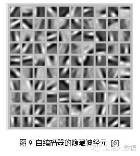
It can be seen that these 100 images have the ability to detect object edges from different orientations. Clearly, this ability is very helpful for subsequent image recognition.
5.2 Restricted Boltzmann Machine (RBM)
A Restricted Boltzmann Machine (RBM) is a bipartite graph, one layer being the input layer (v) and the other layer being the hidden layer (h), assuming that all nodes are random binary variable nodes that can only take values of 0 or 1, and that the full probability distribution p(v, h) satisfies the Boltzmann distribution.
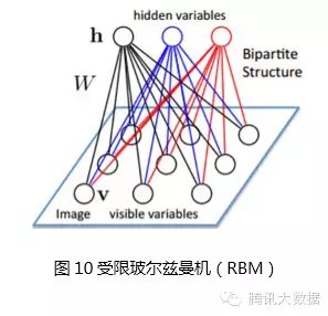
Since there are no connections between nodes of the same layer, given the input layer, the nodes of the hidden layer are conditionally independent; conversely, given the hidden layer, the nodes of the input layer are also conditionally independent. At the same time, according to the Boltzmann distribution, when inputting v, the hidden layer can be generated through p(h|v), and after obtaining the hidden layer, the input layer can be generated through p(v|h). Many readers may have guessed that we can adjust parameters similarly to training other networks, hoping to generate h from input v, and then generate v’ that is as close as possible to v, indicating that the hidden layer h is another representation of the input layer v. This can serve as a basic layer component of deep models. A deep model formed entirely of RBMs is called a Deep Boltzmann Machine (DBM). If the part close to the input layer is replaced with a Bayesian belief network, i.e., a directed graph model, while the part far from the input layer still uses RBM, it is called a Deep Belief Network (DBN).
5.3 Convolutional Neural Networks (CNN)
The encoders introduced above are all fully connected networks, capable of performing 10×10 image recognition, such as handwritten digit recognition. However, for larger images, such as 100×100 images, if we want to learn 100 features, we would need 1,000,000 parameters, which would greatly increase computation time. An effective method for recognizing images of such size is to utilize the locality of images to construct a partially connected network. One of the most common networks is the Convolutional Neural Network (CNN) [15][16], which leverages the inherent property of images: the local statistical properties of an image are the same as those of other locals. Therefore, features learned from a certain local area can also apply to other local areas, and the same features can be used for all positions in the image.
Specifically, suppose there is a 100×100 image, and we want to learn a 10×10 local image feature neuron from it. If we use a fully connected approach, a 100×100-dimensional input to this neuron would require 10,000 connection weight parameters. However, using a convolution kernel, only 10×10 = 100 parameters are needed. The convolution kernel can be seen as a 10×10 small window that moves up, down, left, and right across the image, covering every 10×10 position in the image (there are a total of 91×91 positions). Each time it moves to a position, the input at that position is multiplied with the parameters of the convolution kernel at corresponding positions and summed up to produce an output value (the output value is a 91×91 image). The characteristic of the convolution kernel is that although there are many connections, there are only 10×10 = 100 parameters, significantly reducing the number of parameters, making training easier and less prone to overfitting. Of course, one neuron can only extract one feature; to extract multiple features, multiple convolution kernels are needed.
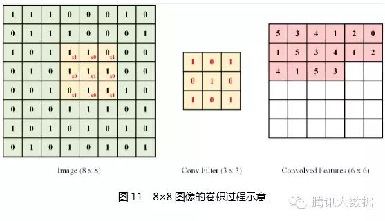
The following figure illustrates the process of using convolution methods to extract features from an 8×8 image. A 3×3 convolution kernel was used, and after moving through every 3×3 position in the image, the final output image obtained is 6×6:
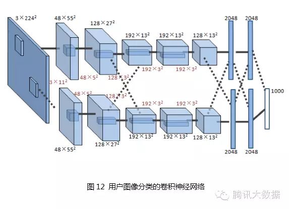
The figure shows the convolutional neural network used by Hinton’s research group in the ImageNet competition [2], which has 5 convolutional layers, with 96, 256, 384, 384, and 256 convolution kernels respectively, and the sizes of the convolution kernels in each layer are 11×11, 5×5, 3×3, 3×3, and 3×3.
6. Training Acceleration of Deep Learning
Training deep models requires various techniques, such as selecting network structures, setting the number of neurons, initializing weight parameters, adjusting learning rates, controlling mini-batches, etc. Even with expertise in these techniques, multiple trainings and repeated explorations are needed in practice. Additionally, deep models have many parameters, a large computational load, and require massive training data, consuming a lot of computational resources. If training can be accelerated, more new ideas can be tried and more parameter groups can be debugged in the same amount of time, significantly improving work efficiency. For large-scale training data and models, it can turn previously impossible tasks into possible ones. This section discusses methods for accelerating the training of deep models.
6.1 GPU Acceleration
Vectorized programming is an effective method for improving algorithm speed. To enhance the speed of specific numerical operations (such as matrix multiplication, matrix addition, matrix-vector multiplication, etc.), researchers in numerical computation and parallel computing have worked for decades. Vectorized programming emphasizes single instruction parallel operations on multiple similar data, forming a programming paradigm of single instruction stream and multiple data streams (SIMD). The algorithms of deep models, such as BP, Auto-Encoder, CNN, etc., can all be written in vectorized form. However, when executed on a single CPU, vector operations will be expanded into loop forms, essentially still executed serially.
GPUs (Graphic Processing Units) have a many-core architecture that contains thousands of stream processors, allowing vector operations to be performed in parallel, greatly shortening computation time. With companies like NVIDIA and AMD continuously advancing their GPU’s large-scale parallel architecture support, General-Purpose GPUs (GPGPU) have become an important means to accelerate parallel applications. Thanks to the many-core architecture of GPUs, programs running on GPU systems are often dozens to thousands of times faster than on single-core CPUs. Currently, GPUs have matured significantly, benefiting the field of scientific computing, with typical successful cases including multi-body problems (N-Body Problem), protein molecular modeling, medical imaging analysis, financial computation, cryptography, etc.
Using GPUs to train deep neural networks can fully leverage their efficient parallel computing capabilities with thousands of computing cores, significantly reducing the time spent in scenarios using massive training data, and requiring fewer servers. If a suitable deep neural network is reasonably optimized, a single GPU card can equal the computational power of dozens or even hundreds of CPU servers, making GPUs the preferred solution in the industry for training deep learning models.
6.2 Data Parallelism
Data parallelism refers to splitting the training data and simultaneously using multiple model instances to train multiple data shards in parallel.
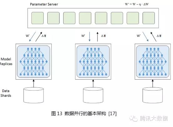
To achieve data parallelism, parameter exchange is needed, typically facilitated by a parameter server. During training, multiple training processes are independent, and the training results, i.e., the changes in the model ΔW, need to be reported to the parameter server, which is responsible for updating the latest model W’ = W – η ∙ ΔW, and then redistributing the latest model W’ to the training programs to start training from the new starting point.
Data parallelism can be divided into synchronous and asynchronous modes. In synchronous mode, all training programs simultaneously train a batch of training data, and after completion, they synchronize and then exchange parameters simultaneously. Once parameter exchange is completed, all training programs have a common new model as a starting point to train the next batch. In asynchronous mode, when a training program completes a batch of training data, it immediately exchanges parameters with the parameter server, disregarding the status of other training programs. In asynchronous mode, the latest results of one training program will not immediately reflect in other training programs until they perform the next parameter exchange.
The parameter server is merely a logical concept and does not necessarily need to be deployed as an independent server. Sometimes it may be attached to a specific training program, and at other times, the parameter server may be partitioned according to the model and deployed separately.
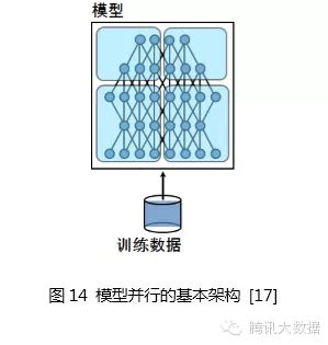
6.3 Model Parallelism
Model parallelism divides the model into several shards, each held by several training units, which work together to complete training. Communication overhead arises when a neuron’s input comes from the output of another neuron’s training unit.
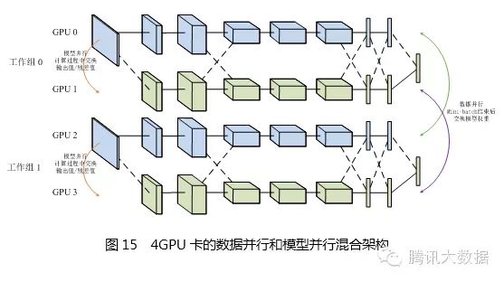
In most cases, the communication overhead and synchronization costs brought by model parallelism exceed those of data parallelism, hence the acceleration ratio is not as good as that of data parallelism. However, for large models that cannot be accommodated in single machine memory, model parallelism is a good choice. Unfortunately, neither data parallelism nor model parallelism can scale indefinitely. When there are too many training programs for data parallelism, the learning rate must be reduced to ensure a smooth training process; when there are too many shards for model parallelism, the amount of neuron output value exchanges will increase sharply, leading to significant efficiency drops. Therefore, a common solution is to conduct both model and data parallelism simultaneously. As shown in the figure below, four GPUs are divided into two groups, with GPUs 0 and 1 as one group for model parallelism, and GPUs 2 and 3 as another group. Each group exchanges output values and residuals during the computation process, while data parallelism occurs between the two groups. After the mini-batch ends, model weights are exchanged, considering that the blue part of the model is held by GPUs 0 and 2, while the yellow part is held by GPUs 1 and 3, thus only the same-colored GPUs need to exchange weights.
6.4 Computing Clusters
Building CPU clusters for training deep neural network models is also a commonly used solution in the industry, leveraging the powerful computing capabilities of large-scale distributed computing clusters to achieve fast training of deep models, utilizing the model’s distributed storage and the asynchronous communication of parameters.
The basic architecture of the CPU cluster scheme includes workers to execute training tasks, a parameter server for distributed storage and distribution of model parameters, and a master program to coordinate the overall tasks. The CPU cluster scheme is suitable for training large models that cannot fit into GPU memory, as well as sparse connection neural networks. Andrew Ng and Jeff Dean at Google trained deep neural networks using model parallelism and Downpour SGD data parallelism on 1,000 CPU servers [17].
Combining GPU computing and cluster computing technologies, constructing GPU clusters is becoming an effective solution to accelerate the training of large-scale deep neural networks. GPU clusters are built on CPU-GPU systems, using faster network communication facilities such as 10 Gigabit network cards or Infiniband, as well as logical network topologies such as tree structures. By fully exploiting the high computational capabilities of single nodes, the collaborative computing capabilities of multiple servers in the cluster can be further utilized to accelerate large-scale training tasks.
7. Software Tools and Platforms for Deep Learning
Currently, there are many relatively mature software tools and platforms for implementing deep learning systems.
7.1 Open Source Software
In the open-source community, several mature software tools include:
Kaldi is a speech recognition toolkit based on C++ and CUDA [18][19], provided for researchers in speech recognition. Kaldi implements both single GPU accelerated deep neural network SGD training and CPU multi-threaded accelerated deep neural network SGD training.
Cuda-convnet is written in C++/CUDA and implements deep convolutional neural networks using the backpropagation algorithm [20][21]. Released in 2012, cuda-convnet supports training on a single GPU, and the deep convolutional neural network model trained based on it achieved a Top 5 classification error rate of 15% on ImageNet LSVRC-2012 [2]; the version released in 2014 supports data parallel and model parallel training on multiple GPUs [22].
Caffe provides fast implementations of convolutional neural networks on both CPU and GPU, along with training algorithms, allowing training of over 40,000,000 images in a day using NVIDIA K40 or Titan GPUs [23][24].
Theano provides a Python library for mathematical computations in deep learning, integrating the NumPy matrix computation library, capable of running on GPUs and offering good algorithmic extensibility [25][26].
OverFeat is a convolutional neural network system developed by New York University’s CILVR lab, primarily used for image recognition and feature extraction [27].
Torch7 is a scientific computing framework that provides extensive support for machine learning algorithms, with its neural network toolkit (Package) implementing basic modules such as mean squared error cost function, nonlinear activation functions, and gradient descent training algorithms for neural networks, allowing easy configuration of target multi-layer neural networks for training experiments [28].
7.2 Industrial Platforms
In the industry, companies like Google, Facebook, Baidu, and Tencent have implemented their own software frameworks:
Google’s DistBelief system is a data parallel and model parallel framework implemented on CPU clusters, using tens of thousands of CPU cores to train deep neural network models with up to 1 billion parameters. The main algorithms used in DistBelief include Downpour SGD and L-BFGS, with supported applications in speech recognition and image classification of 21,000 categories [17].
Google’s COTS HPC system is a data parallel and model parallel framework implemented on GPUs, connecting GPU servers using Infiniband and controlling communication via MPI. COTS can complete training of deep neural networks with 1 billion parameters in a few days using three GPU servers [29].
Facebook has implemented a parallel framework for multi-GPU training of deep convolutional networks, combining data parallelism and model parallelism to train CNN models, using four NVIDIA Titan GPUs to train the ImageNet 1000 classification network in a few days [30].
Baidu has built the Paddle (Parallel Asynchronous Distributed Deep Learning) multi-machine GPU training platform [31]. It distributes data across different machines and coordinates training through a Parameter Server. Paddle supports both data parallelism and model parallelism.
Tencent’s deep learning platform (Mariana) was developed to accelerate the training of deep learning models, including multi-GPU data parallel frameworks for deep neural networks, multi-GPU model parallel and data parallel frameworks for deep convolutional networks, and CPU cluster frameworks for deep neural networks. Mariana designs customized parallel training platforms based on specific application training scenarios, supporting speech recognition, image recognition, and actively exploring applications in advertising recommendations [32].
8. Conclusion
In recent years, the field of artificial intelligence has witnessed a wave of deep learning, with enthusiasm soaring from academia to industry. Deep learning attempts to solve the problem of abstract cognition in artificial intelligence, achieving significant success in both theoretical analysis and applications. It can be said that deep learning is currently the most intelligent learning method closest to the human brain.
Deep learning can achieve complex function approximation by learning a deep nonlinear network structure, demonstrating a powerful ability to learn the essence of datasets and highly abstract features. Training methods such as layer-wise initialization have significantly improved the learnability of deep models. Compared to traditional shallow models, deep models undergo several layers of nonlinear transformations, providing strong expressive capabilities for modeling more complex tasks. Compared to manual feature engineering, automatically learned features can better mine the rich inherent information in the data and have stronger scalability. Deep learning aligns with the trend of big data, and with sufficient training samples, complex deep models can fully unleash their potential, mining the rich information contained in massive data. Strong foundational infrastructure and customized parallel computing frameworks have made previously unimaginable training tasks accelerate completion, laying a solid foundation for the practical application of deep learning. There are already multiple open-source implementations for different deep models, such as Kaldi, Cuda-convnet, and Caffe, and companies like Google, Facebook, Baidu, and Tencent have also implemented their own parallelization frameworks.
The revolution ignited by deep learning has brought artificial intelligence to a new level, with not only significant academic meaning but also strong practicality. Deep learning will become the powerful technological engine behind a large number of products and services.
References
[1] Geoffery E. Hinton, Salakhutdinov RR. Reducing the dimensionality of data with neural networks. Science. 2006 Jul 28;313(5786):504-7.
[2] ImageNet Classification with Deep Convolutional Neural Networks, Alex Krizhevsky, Ilya Sutskever, Geoffrey E Hinton, NIPS 2012.
[3] Q.V. Le, M.A. Ranzato, R. Monga, M. Devin, K. Chen, G.S. Corrado, J. Dean, A.Y. Ng. Building high-level features using large scale unsupervised learning. ICML, 2012.
[4] Rick Rashid, Speech Recognition Breakthrough for the Spoken, Translated Wordhttp://www.youtube.com/watch?v=Nu-nlQqFCKg
[5] NYU “Deep Learning” Professor LeCun Will Lead Facebook’s New Artificial Intelligence Lab.http://techcrunch.com/2013/12/09/facebook-artificial-intelligence-lab-lecun/
[6] Stanford deep learning tutorialhttp://deeplearning.stanford.edu/wiki/index.php/UFLDL_Tutorial
[7] A Primer on Deep Learninghttp://www.datarobot.com/blog/a-primer-on-deep-learning/
[8] The Nobel Prize in Physiology or Medicine 1981.http://www.nobelprize.org/nobel_prizes/medicine/laureates/1981/
[9] Bruno A. Olshausen & David J. Field, Emergence of simple-cell receptive field properties by learning a sparse code for natural images. Nature. Vol 381. 13 June, 1996http://www.cs.ubc.ca/~little/cpsc425/olshausen_field_nature_1996.pdf
[10] Back propagation algorithm http://ufldl.stanford.edu/wiki/index.php/Backpropagation_Algorithm
[11] 余凯,深度学习-机器学习的新浪潮,Technical News程序天下事http://blog.csdn.net/datoubo/article/details/8577366
[12] Support Vector Machine http://en.wikipedia.org/wiki/Support_vector_machine
[13] Logistic Regression http://en.wikipedia.org/wiki/Logistic_regression
[14] Deep Networks Overview http://ufldl.stanford.edu/wiki/index.php/Deep_Networks:_Overview
[15] Y. LeCun and Y. Bengio. Convolutional networks for images, speech, and time-series. In M. A. Arbib, editor, The Handbook of Brain Theory and Neural Networks. MIT Press, 1995
[16] Introduction to Convolutional neural networkhttp://en.wikipedia.org/wiki/Convolutional_neural_network
[17] Dean, J., Corrado, G.S., Monga, R., et al, Ng, A. Y. Large Scale Distributed Deep Networks. In Proceedings of the Neural Information Processing Systems (NIPS’12) (Lake Tahoe, Nevada, United States, December 3–6, 2012). Curran Associates, Inc, 57 Morehouse Lane, Red Hook, NY, 2013, 1223-1232.
[18] Kaldi project http://kaldi.sourceforge.net/
[19] Povey, D., Ghoshal, A. Boulianne, G., et al, Vesely, K. Kaldi. The Kaldi Speech Recognition Toolkit. in Proceedings of IEEE 2011 Workshop on Automatic Speech Recognition and Understanding(ASRU 2011) (Hilton Waikoloa Village, Big Island, Hawaii, US, December 11-15, 2011). IEEE Signal Processing Society. IEEE Catalog No.: CFP11SRW-USB.
[20] cuda-convent https://code.google.com/p/cuda-convnet/
[21] Krizhevsky, A., Sutskever, I., and Hinton, G.E. ImageNet Classification with Deep Convolutional Neural Networks. In Proceedings of the Neural Information Processing Systems (NIPS’12) (Lake Tahoe, Nevada, United States, December 3–6, 2012). Curran Associates, Inc, 57 Morehouse Lane, Red Hook, NY, 2013, 1097-1106.
[22] Krizhevsky, A. Parallelizing Convolutional Neural Networks. in tutorial of IEEE Conference on Computer Vision and Pattern Recognition (CVPR 2014). (Columbus, Ohio, USA, June 23-28, 2014). 2014.
[23] caffe http://caffe.berkeleyvision.org/
[24] Jia, Y. Q. Caffe: An Open Source Convolutional Architecture for Fast Feature Embedding.http://caffe.berkeleyvision.org (2013).
[25] Theano https://github.com/Theano/Theano
[26] J. Bergstra, O. Breuleux, F. Bastien, P. Lamblin, R. Pascanu, G. Desjardins, J. Turian, D. Warde-Farley and Y. Bengio. Theano: A CPU and GPU Math Expression Compiler. Proceedings of the Python for Scientific Computing Conference (SciPy) 2010. June 30 – July 3, Austin, TX.
[27] Overfeat http://cilvr.nyu.edu/doku.php?id=code:start
[28] Torch7 http://torch.ch
[29] Coates, A., Huval, B., Wang, T., Wu, D. J., Ng, A. Y. Deep learning with COTS HPC systems. In Proceedings of the 30th International Conference on Machine Learning (ICML’13) (Atlanta, Georgia, USA, June 16–21, 2013). JMLR: W&CP volume 28(3), 2013, 1337-1345.
[30] Yadan, O., Adams, K., Taigman, Y., Ranzato, M. A. Multi-GPU Training of ConvNets. arXiv:1312.5853v4 [cs.LG] (February 2014)
[31] Kaiyu, Large-scale Deep Learning at Baidu, ACM International Conference on Information and Knowledge Management (CIKM 2013)
[32] aaronzou, Mariana深度学习在腾讯的平台化和应用实践
[33] Geoffrey E. Hinton, Simon Osindero, Yee-Whye Teh, A fast learning algorithm for deep belief nets Neural Compute, 18(7), 1527-54 (2006)
[34] Andrew Ng. Machine Learning and AI via Brain simulations,https://forum.stanford.edu/events/2011slides/plenary/2011plenaryNg.pdf
[35] Geoffrey Hinton:UCLTutorial on: Deep Belief Nets
[36] Krizhevsky, Alex. “ImageNet Classification with Deep Convolutional Neural Networks”. Retrieved 17 November 2013.
[37] “Convolutional Neural Networks (LeNet) – DeepLearning 0.1 documentation”. DeepLearning 0.1. LISA Lab. Retrieved 31 August 2013.
[38] Bengio, Learning Deep Architectures for AI,http://www.iro.umontreal.ca/~bengioy/papers/ftml_book.pdf;
[39] Deep Learning http://deeplearning.net/
[40] Deep Learning http://www.cs.nyu.edu/~yann/research/deep/
[41] Introduction to Deep Learning. http://en.wikipedia.org/wiki/Deep_learning
[42] Google的猫脸识别:人工智能的新突破http://www.36kr.com/p/122132.html
[43] Andrew Ng’s talk video: http://techtalks.tv/talks/machine-learning-and-ai-via-brain-simulations/57862/
[44] Invited talk “A Tutorial on Deep Learning” by Dr. Kai Yu http://vipl.ict.ac.cn/News/academic-report-tutorial-deep-learning-dr-kai-yu