
Author: Zhang Xu
Editor: Wang Shuwei
This article has 4794 words and 27 images, reading time is about 11 minutes
Forget it
Read as long as you want

1. Convolutional Layer
1.1 The Role of Convolutional Layer in CNN
1.2 How Convolutional Layers Work
1.3 Convolutional Layers in AlexNet
2. Pooling and Activation Layers
2.1 Pooling Layer
2.2 Activation Layer
3. Fully Connected Layer
3.1 The Role of Fully Connected Layer
3.2 Fully Connected Layers in AlexNet
4. Softmax Layer
4.1 The Role of Softmax
4.2 Softmax in AlexNet
5. 60M Parameters in AlexNet
6. Development of CNN
Background:
In 2012, AlexNet won the ImageNet competition. Although many faster and more accurate convolutional neural network structures have emerged since then, AlexNet, as a pioneer, still has many aspects worth learning from. Below, we will dissect AlexNet to understand the general structure of convolutional neural networks.
First, let’s look at some parameters and structure of AlexNet: Convolutional Layers: 5 layers Fully Connected Layers: 3 layers Depth: 8 layers Number of Parameters: 60M Number of Classes: 1000
Structure Diagram:
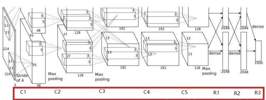
Due to the limitations of GPU memory at that time, AlexNet’s 60M parameters could not all be processed on a single GPU, so two GPUs were used to operate separately, with interactions occurring at layers C3, R1, R2, and R3. This interaction, known as channel merging, is a type of concatenation operation.
Convolutional Layer:
1.1 The Role of Convolutional Layer in CNN::
In CNN, the convolutional layer is often represented as conv, which is short for convolution.
The convolutional layer plays a crucial role in CNN—feature abstraction and extraction. This is a significant difference between CNN and traditional ANN or SVM. In traditional machine learning algorithms, I need to manually specify what the features are.
For example, the classic HOG+SVM pedestrian detection scheme uses HOG as a feature extraction method.
Thus, what we input into the SVM classifier are the features extracted by HOG, not the images themselves. Therefore, sometimes the choice of feature extraction algorithm is more important than the classification model.
In CNN, the feature extraction work is automatically completed in the convolutional layer. Generally, the deeper and wider the convolutional layer, the better its expressive ability. Therefore, CNN allows for end-to-end training, where we input raw data, not manually extracted features.
From this perspective, CNN can be seen as a self-learning feature extractor + softmax classifier (not considering the fully connected logical judgment layer at this point, as it was later removed).
1.2 How Convolutional Layers Work:
The operation of convolutional layers in CNN is the same as that of convolution in image processing, which involves a convolution kernel performing a weighted summation operation from top to bottom and from left to right. The difference is that in traditional image processing, we manually specify the convolution kernel, such as Sobel, which can extract horizontal and vertical edges in an image.
In CNN, the size of the convolution kernel is specified manually, but all the numbers within the convolution kernel need to be learned continuously.
For example, if a convolution kernel has a size of 3*3*3, it has 27 parameters (width, height, depth).
It is important to clarify one point:
Thickness of Convolution Kernel = Number of Channels in the Convolved Image Number of Convolution Kernels = Number of Output Channels after Convolution
This relationship is crucial for understanding the convolutional layer!!
For example, if the input image size is 5*5*3 (width/height/channels), convolution kernel size: 3*3*3 (width/height/thickness), stride: 1, padding: 0, number of convolution kernels: 1.
Using such a convolution kernel on a specific position of the image will multiply the 27 pixel values at that position (3 width, 3 height, 3 channels) by the corresponding parameters of the convolution kernel and obtain a single number. This process is repeated as the kernel slides over the image to produce the convolved image, which has one channel (the same as the number of convolution kernels). The height and width of the convolved feature can be calculated using the formula: (5-3+2*0)/1 +1 = 3, resulting in a feature size of: 3*3*1 (width/height/channels).
1.3 Convolutional Layers in AlexNet:
In AlexNet, the convolutional layers are represented as C1…C5, totaling 5 layers. Each convolution result can be seen in the diagram; for instance, after passing through the C1 layer, the original image size becomes 55*55 with a total of 96 channels, distributed across 2 GPUs with 3GB memory each.
Thus, the size of the cube in the diagram is 55*55*48, where 48 is the number of channels (which will be explained in detail later). Inside this cube, there is also a smaller cube of size 5*5*48, which represents the kernel size of the C2 convolutional layer, where 48 is the thickness of the kernel (to be explained later).
We can see the kernel sizes for each layer and the dimensions of the output after each convolution. Following the previous explanation, we can derive the convolution operations for each layer:
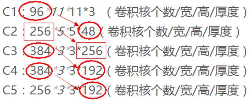
Input Layer: 224*224*3 C1: 96*11*11*3 (number of kernels/width/height/thickness) C2: 256*5*5*48 (number of kernels/width/height/thickness) C3: 384*3*3*256 (number of kernels/width/height/thickness) C4: 384*3*3*192 (number of kernels/width/height/thickness) C5: 256*3*3*192 (number of kernels/width/height/thickness)
Regarding these five convolutional layers, three points should be noted: 1. Derive the output after C1: Using an 11*11*3 convolution kernel to convolve a 224*224*3 image, the output size after convolution is 55*55*1.
Because: (224-11+3)/4+1=55
The number of convolution kernels is 96, but 48 are on one GPU, while the remaining 48 are on another GPU.
Thus, the number of channels on a single GPU is 48, multiplied by 2 for the number of GPUs.
The final output is: 55*55*48*2, and the remaining layers follow the same derivation process as above.
2. Note the pooling operations during the derivation: After the convolution operations in C1, C2, and C5, the image undergoes max pooling (to be discussed later), which affects the size of the output image. 3. The uniqueness of the C3 convolutional layer:
Looking at the above diagram, due to the separate GPU operations, the number of output channels from the previous layer (which is also the number of convolution kernels) is always twice the thickness of the convolution kernels in the next convolution layer.
However, C3 is special—why is that??
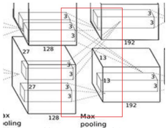
Because here, channel merging occurs, which is a type of concatenation operation. Thus, a convolution kernel does not convolve only the image from a single GPU, but rather the image from both GPUs concatenated together. After concatenation, the number of channels is 256, so the thickness of the convolution kernel is 256.
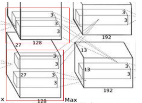
This is why there are two 3*3*128 convolution kernels drawn in this diagram; it means that the actual convolution kernel size is 3*3*256! (This conclusion is based on personal understanding)
Pooling and Activation Layers:
Strictly speaking, pooling and activation layers do not belong to separate layers in CNN and are not counted in the total number of CNN layers. Therefore, we generally say that AlexNet has a total of 8 layers, consisting of 5 convolutional layers and 3 fully connected layers.
However, for clarity, we separate them out for explanation.
2.1 Pooling Layer:
Pooling operations (Pooling) are used after convolution operations, serving to fuse features and reduce dimensionality. It is similar to convolution, but all parameters in the pooling layer are hyperparameters and do not need to be learned.
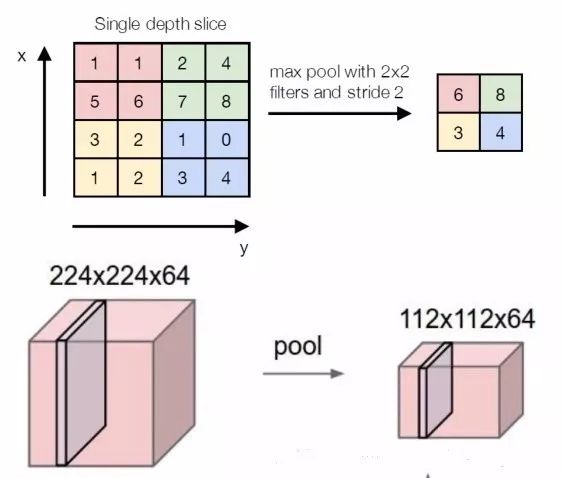
The above image explains the process of max pooling, where the kernel size is 2*2 and the stride is 2. The max pooling process takes the maximum value within the 2*2 area as the pixel value for the output channel.
In addition to max pooling, there is also average pooling, which instead of taking the maximum, takes the average.
For an input image of size 224*224*64, after max pooling, the size becomes 112*112*64, demonstrating that pooling operations change the width and height of the image but do not alter the number of channels.
2.2 Activation Layer:
Pooling operations are used within convolutional layers, while activation operations are utilized in both convolutional and fully connected layers. Here, we will briefly explain it; specific content can be found in the blog on understanding the role of activation functions in neural network model construction. Generally, in deep networks, the ReLU piecewise linear function is used as the activation function, as shown in the figure below, which increases non-linearity.
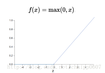
The activation process in fully connected layers is easy to understand since the output of all neurons in a fully connected layer is a single number. If this number x>0, then x=x; if x<0, then x=0.
The activation in convolutional layers targets each pixel value. For example, if a certain pixel value at row i and column j in a channel of the output from a convolutional layer is x, then if x>0, then x=x; if x<0, then x=0.
Fully Connected Layer:
3.1 The Role of Fully Connected Layer:
The role of fully connected layers in CNN is the same as in traditional neural networks, responsible for logical inference, with all parameters needing to be learned.
One difference is that the first fully connected layer links to the output of the convolutional layers and also serves to remove spatial information (number of channels), transforming a three-dimensional matrix into a vector (a type of fully convolutional operation), as shown below:
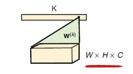
If the input image is W*H*C, and the convolution kernel size is W*H*C, the entire input image will be transformed into a single number, resulting in k numbers (the number of neurons after the first fully connected layer). Therefore, there are K convolution kernels of size W*H*C.
Thus, the parameter count in fully connected layers (especially the first layer) is significantly large. Due to this drawback, later networks eliminated fully connected layers, which will be discussed further if given the chance.
3.2 Fully Connected Layers in AlexNet:
Returning to the structure of AlexNet, R1, R2, and R3 are the fully connected layers.
R2 and R3 are straightforward, but here we mainly explain R1 layer: Input image: 13*13*256 Convolution kernel size: 13*13*256 Number: 2048*2 Output size: 4096 (column vector) From the initial structure, we can see that R1 also has channel interactions:
Thus, the concatenated channel count is 256, and the size of the fully convolutional kernels is 13*13*256. Each of the 4096 kernels performs a full convolution operation on the input image, resulting in a column vector with 4096 numbers.
The arrangement of these numbers is equivalent to the first hidden layer in a traditional neural network. After R1, the connection method for subsequent layers is no different from that of an ANN. The parameters to be learned have shifted from convolution kernel parameters to weight coefficients in fully connected layers.
Softmax Layer:
4.1 The Role of Softmax:
The Softmax layer is not a separate layer in CNN. Generally, when using CNN for classification, the common practice is to convert the outputs of neurons into probabilities, and Softmax performs this function:
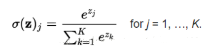
This is easy to understand; clearly, the outputs of the Softmax layer sum to 1. The value of any single output represents the probability, and we determine the class based on the size of this probability.
4.2 Softmax in AlexNet:
The final classification number of AlexNet is 1000, meaning the final output is 1000, with an input of 4096, linked through R3, which is the last layer, the third fully connected layer, and the eighth layer overall. This concludes the entire structure of AlexNet!
60M Parameters in AlexNet:
AlexNet has only 8 layers, but it requires learning 60,000,000 (consider the magnitude of this number) parameters, which is quite a daunting figure compared to the number of layers.
Let’s calculate how these parameters are derived:
C1: 96*11*11*3 (number of kernels/width/height/thickness) 34848 C2: 256*5*5*48 (number of kernels/width/height/thickness) 307200 C3: 384*3*3*256 (number of kernels/width/height/thickness) 884736 C4: 384*3*3*192 (number of kernels/width/height/thickness) 663552 C5: 256*3*3*192 (number of kernels/width/height/thickness) 442368 R1: 4096*6*6*256 (number of kernels/width/height/thickness) 37748736 R2: 4096*4096 16777216 R3: 4096*1000 4096000
In R1, the kernel size is 6*6*256 instead of 13*13*256 because it underwent max pooling. It can be seen that the fully connected layer (especially the first layer) accounts for the majority of the parameter count.
Development of CNN:
Since the advent of AlexNet, CNN has developed rapidly. By 2016, multiple generations of network structures have emerged, with increasing depth and width, improving efficiency and accuracy: LeNet5—AlexNet—NiN—VGG—GoogleNet—ResNet—DenseNet. Among these structures:
NiN introduced 1*1 convolution layers (Bottleneck layer) and global pooling; VGG replaced 7*7 convolution kernels with three 3*3 convolution kernels, reducing parameters; GoogLeNet introduced the Inception module; ResNet introduced the concept of residual connections;
DenseNet further improved on ResNet’s direct connection concept by connecting the output features of the current layer to all subsequent layers.
Some networks have removed certain ideas proposed in AlexNet, such as fully connected layers and full-size convolutions, but AlexNet, and even earlier LeNet5, have played a milestone role in the development of CNN.
PS:
If you have some knowledge of ANN, that’s better. If not, leave a message to the editor, and I will help you build a solid foundation.
Thank you all for supporting the public account
For questions related to CNN knowledge and other issues
Everyone is welcome to join the group for discussions.
Feel free to leave messages or appreciate.
Recommended
Read
Learn
-
Master machine learning, here is everything you need
-
Interesting discussions on the core of deep learning—activation functions
-
Practical article on Naive Bayes for Sina News classification
-
Object Detection R-CNN