An Explanation and Derivation of the XGBoost Algorithm

This article is excerpted from “Introduction to Machine Learning Basics (Micro Course Version)”

10.5 XGBoost Algorithm

XGBoost is a machine learning algorithm based on the gradient boosting algorithm (GBDT) invented by PhD student Tianqi Chen from the University of Washington in February 2014. This algorithm not only has excellent learning performance but also trains efficiently, shining in data competitions.

XGBoost is a tool for large-scale parallel Boosting Tree, which is an open-source Boosting Tree toolkit with both performance and speed that is many times faster than commonly used toolkits. Both XGBoost and GBDT are Boosting methods, and aside from some differences in engineering implementation and problem-solving, the biggest difference is the definition of the objective function.

10.5.1 Algorithm Principles

The principles of the XGBoost algorithm mainly involve the following aspects:

1. Prevent Overfitting

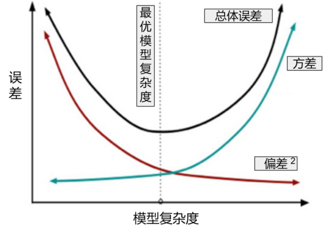
The generalization error of machine learning algorithms can be divided into bias and variance. Bias refers to the degree of deviation between the expected prediction and the actual prediction of the algorithm, reflecting the model’s fitting ability; variance measures the variation in learning performance caused by changes in a training set of the same size, depicting the impact of data perturbation.

As shown in Figure 10-9, as the complexity of the machine learning model increases, bias decreases, but variance increases. When the model is simpler, variance is small, but bias tends to be larger, meaning that high variance leads to overfitting, while high bias leads to underfitting.

XGBoost effectively addresses the overfitting problem by penalizing the weights of leaf nodes, preventing overfitting, which is equivalent to adding a regularization term, i.e., the objective function is: training loss plus the regularization term.

2. Use Second-Order Taylor Expansion to Accelerate Convergence

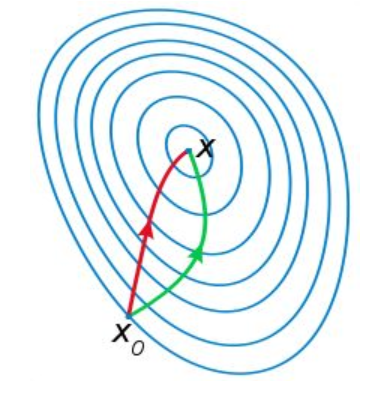
The loss function of GBDT uses first-order convergence and employs gradient descent, while XGBoost uses Newton’s method for second-order convergence, i.e., it performs a second-order Taylor expansion of the loss function and uses the first two orders as improved residuals. The gradient descent method uses the first derivative of the objective function, while Newton’s method uses the second derivative of the objective function. The second derivative considers the trend of change in the gradient, making it easier for Newton’s method to converge. Figure 10-10 shows the iterative paths of Newton’s method (left) and gradient descent (right), where the left path better aligns with the optimal descent path. Using second-order convergence is also the reason why XGBoost accelerates convergence.

3. Split Criteria for Tree Construction Use Derivative Statistics

When searching for the best split point, XGBoost implements a fully searching, precise greedy algorithm (Exact Greedy Algorithm). This search algorithm traverses all possible split points on a feature, calculates the loss reduction for each, and then selects the optimal split point. The importance of a feature is determined by the total number of times it appears across all trees. After calculating the gain, the feature with the highest gain is selected for splitting, and its importance is incremented by one.

4. Supports Parallel Computing and Can Use Multi-threaded Optimization Techniques

The parallelism in XGBoost does not mean that each tree can be trained in parallel. XGBoost fundamentally still adopts the boosting idea; each tree needs to wait for the previous tree to complete training before starting training.

The parallelism in XGBoost refers to the parallelism in feature dimensions: before training, each feature is pre-sorted by its feature values and stored in a Block structure, which can be reused later when searching for feature split points. Since features are stored as individual block structures, multi-threading can be utilized to compute the best split point for each block in parallel.

10.5.2 Derivation of the XGBoost Algorithm

The main base learner in XGBoost is CART (Classification and Regression Trees). Here, let the weight of the leaf be defined as , the function that assigns each node to a leaf as , the number of trees as , and define as a constant. Assuming the model optimized in the previous iterations is , the target function for the step is:

In formula (10.14), the first part is the training error between the predicted value and the true target value, and the second part is the sum of the complexities of each tree.

According to the Taylor expansion formula, a second-order Taylor expansion is used:

Let be treated as , then can be seen as . Thus:

In the above formula:

is the first derivative of ;

is the second derivative of ;

Then formula (10.14) can be transformed into:

Here, we first redefine a tree as follows:

In XGBoost, we define the complexity as:

Thus, the objective function can be defined as:

It is clear that is a constant and can be replaced with , which does not affect the objective function, so the objective function can be transformed into:

where is the index set of data points assigned to the th leaf. Since all data points in the same leaf have the same score, we modified the total sum’s index in the second line. Therefore, the formula is equivalent to:

That is:

We can further compress the expression by defining , then:

Taking the derivative with respect to , if there is a given tree structure , then in the case of minimizing the above expression (i.e., the derivative is 0), we get:

Thus:

And obtain the corresponding optimal objective function value:

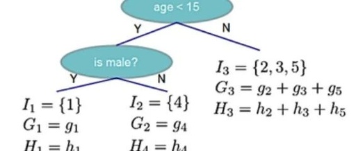
Taking Figure 10-11 as an example:

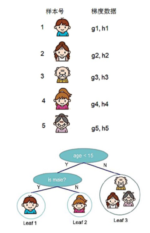
Based on the known data, corresponding parameters are obtained as shown in Figure 10-12:

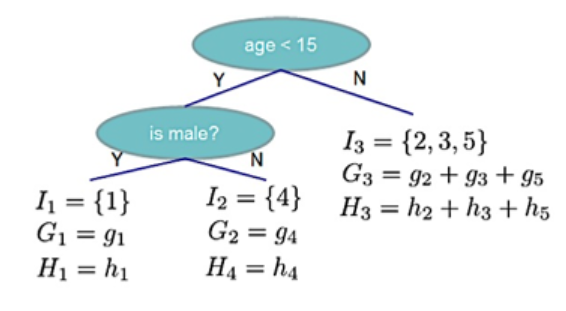
For the data in Figure 10-12, according to formula (10.30), we have:

The smaller the score, the better the structure of this tree.

When searching for the best split point, an exact greedy algorithm (Exact Greedy Algorithm) is used. This search algorithm traverses all possible split points on a feature, calculates the loss reduction for each, and then selects the optimal split point. The process of the exact greedy algorithm is shown in Algorithm 10.1.

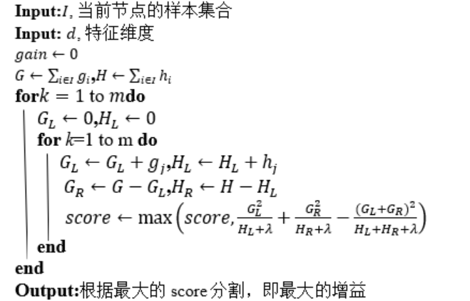
Algorithm Idea: Since the structure of the tree is unknown, and it is impossible to traverse all tree structures, XGBoost uses a greedy algorithm to split nodes, starting from the root node, traversing all attributes, and examining possible values of the attributes. The complexity is: the number of leaf nodes in the decision tree minus 1. According to the definition, let the sample sets scored to the left and right subtrees be , then the loss reduction caused by splitting this node is:

That is:

Where: is the score of the left subtree after the split, is the score of the right subtree after the split, is the score of the unpartitioned tree, and is the regularization term introduced by adding new leaf nodes, we want to find an attribute and its corresponding size such that takes the maximum value.

10.5.3 Summary of the XGBoost Algorithm

XGBoost is one of the most popular algorithms in algorithm competitions, taking the optimization of GBDT to an extreme:

(1) The CART tree generated by XGBoost considers the complexity of the tree, which GBDT does not consider; GBDT considers the complexity of the tree during the pruning step.

(2) XGBoost fits the second derivative expansion of the loss function from the previous round, while GBDT fits the first derivative expansion of the loss function from the previous round. Therefore, XGBoost has higher accuracy and requires fewer iterations to achieve the same training effect.

(3) Both XGBoost and GBDT iteratively improve model performance, but XGBoost can utilize multi-threading to select the best split point, greatly improving running speed. Of course, later Microsoft released LightGBM, which optimized memory usage and running speed, but in terms of the algorithm itself, the optimization points are not more than those of XGBoost.