Understanding XGBoost: A Comprehensive Guide

XGBoost is a hot algorithm suitable for analyzing abstract data problems, achieving great results in competitions like Kaggle. Although there are many articles introducing the principles and use of XGBoost, few can clearly and thoroughly explain its principles. The goal of this article is to systematically and deeply explain the principles of XGBoost, helping everyone truly understand the algorithm’s principles. This article is a supplement to “Machine Learning and Applications” (written by Lei Ming), which has been published by Tsinghua University Press. This book systematically explains the principles and implementations of ensemble learning, bagging and random forests, boosting, and various AdaBoost algorithms. The derivations of AdaBoost and gradient boosting, as well as XGBoost, require the use of generalized additive models, which are also deeply introduced.

Understanding the principles of XGBoost requires basic knowledge of decision trees (especially classification and regression trees), ensemble learning, generalized additive models, and Newton’s method. The decision tree has been thoroughly explained in the previous public account article “Understanding Decision Trees” before SIGAI. Ensemble learning has been discussed in earlier public account articles “Overview of Random Forests”, “Talking about AdaBoost Algorithm”, and “Understanding AdaBoost Algorithm”. Newton’s method has been introduced in previous public account articles “Understanding Gradient Descent Method”, “Understanding Convex Optimization”, and “Understanding Newton’s Method”. If readers are not clear about these concepts, it is recommended to read those articles first.

Decision trees are an old algorithm in machine learning, which can be seen as a set of nested decision rules learned from training. Mathematically, a decision tree is a piecewise constant function, where each leaf node corresponds to a region in the space, and vectors x falling into this region are predicted to have the value of that leaf node.

Classification and regression trees are a type of binary decision tree that can be used for both classification and regression problems. The core problem to solve during training is to find the best split to determine the internal nodes and recursively build the tree, assigning label values to the leaf nodes. For classification problems, the goal when searching for the best split is to maximize the Gini impurity, simplified to the following formula:

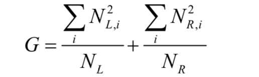
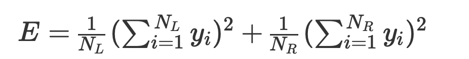
where NL is the number of training samples in the left child node after the split, NL,i is the number of samples of the i-th class in the left child node; NR is the number of training samples in the right child node after the split, NR,i is the number of samples of the i-th class in the right child node. For regression problems, the goal when searching for the best split is to maximize the decrease in regression error.

Because there are multiple features in the feature vector, it is necessary to calculate the best split threshold for each feature component during implementation and select the optimal one. To calculate the best split threshold for a single feature, first sort all training samples at that node in ascending order according to that feature component, then take each feature value as a threshold to split the sample set into two subsets, and calculate the above split metric to find the optimal value. The specific principles are detailed in the book “Machine Learning and Applications”.

The second issue is setting the values of the leaf nodes. For classification problems, the value of the leaf node is set to the class that appears most frequently in the training sample set of that node; for regression trees, it is set to the mean of the label values of the training samples at that node.

Ensemble learning is a major class of algorithms in machine learning, representing a simple idea: combining multiple machine learning models to create a stronger model. The models being combined are called weak learners, while the combined model is called a strong learner. Various algorithms have emerged based on different combination strategies. The most commonly used are bagging and boosting. The representative work of the former is random forests, while the latter includes AdaBoost, gradient boosting, and XGBoost.

In the combination scheme of weak learners, if addition is used to sum the prediction functions of multiple weak learners to obtain a strong learner, it is called a generalized additive model. The objective function fitted by the generalized additive model is a linear combination of multiple basis functions.

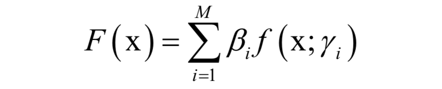
where γi is the parameter of the basis function, βi is the weight coefficient of the basis function. The goal during training is to determine the parameters and weight values of the basis functions; if decision trees serve as basis functions, the parameters include comparing features, comparing thresholds, and leaf node values. The goal during training is to minimize the loss function for all samples.

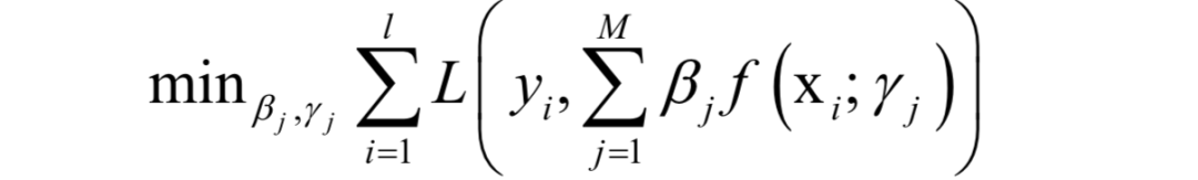
The training algorithm adopts a stepwise refinement strategy, determining the parameters and weights of each basis function sequentially, and then adding them to the strong learner, thereby improving the accuracy of the strong learner. In practical implementation, the output values of the already obtained strong learner for the training samples are treated as constants. Then, a stage-wise optimization strategy is employed, first fixing the weight values βi, optimizing the weak learner. Then the weak learner is treated as a constant to optimize the weight values βi.

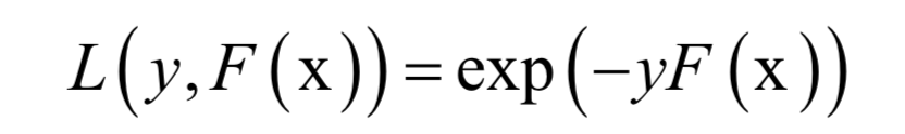
Using the AdaBoost algorithm as an example, the loss of the strong classifier for a single training sample is given by the exponential loss function.

Substituting the prediction function of the generalized additive model into the above loss function yields the objective function to be optimized during algorithm training.

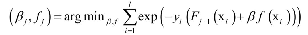
Here the exponential function is split into two parts: the existing strong classifier Fj–1, and the loss function of the current weak classifier f for the training samples, the former has already been determined in previous iterations, thus Fj–1 (xi ) can be considered a constant. Therefore, the objective function can be simplified to.

where

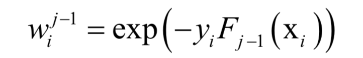
It only relates to the strong classifier obtained from previous iterations and is independent of the current weak classifier or its weight; this is the sample weight of the AdaBoost algorithm. This problem can be solved in two steps: first treating β as a constant, optimizing f(xi); then fixing f(xi) and optimizing β. Thus, the training algorithm of AdaBoost is obtained.

From the generalized additive model, various AdaBoost algorithms can be derived, where their weak classifiers are different, and the objective function optimized during training is also different, including:

The principles of various AdaBoost algorithms and the generalized additive model are detailed in the book “Machine Learning and Applications”; due to space limitations, I will not elaborate here.

In addition to the AdaBoost algorithm, boosting also has other implementation algorithms, such as the gradient boosting algorithm. The gradient boosting algorithm adopts a different approach, also using the generalized additive model, but employs the steepest descent method (a variant of gradient descent) during the solution process. Each weak learner is trained sequentially, but no weights are added to the training samples; instead, pseudo-label values are calculated, which are the negative values of the derivative of the loss function with respect to the predicted values of the training samples obtained by the already determined strong learner Fj–1 (xi ):

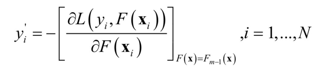
Then the weak learner to be trained in this iteration is used to fit this target. In practical implementation, it is divided into two steps: training the weak learner and searching for the optimal step length (line search).

Newton’s method is a numerical optimization (approximate solution) algorithm for finding the extreme values of functions. According to Fermat’s theorem in calculus, a necessary condition for a function to achieve an extreme value at point x* is that the derivative (for multivariable functions, the gradient) is 0, that is:

Let x* be the stationary point of the function. Therefore, the extreme value of the function can be found by locating its stationary points. Directly calculating the gradient of the function and solving the above equation is generally very difficult; if the function is a complex nonlinear function, this equation is a nonlinear system, which is not easy to solve. Therefore, most people use iterative methods for approximate calculations. It starts from an initial point x0 and repeatedly moves according to certain rules from xk to the next point xk+1 until reaching the extreme point of the function. These rules generally utilize first-order derivative information, i.e., the gradient; or second-order derivative information, i.e., the Hessian matrix. Newton’s method uses both first-order and second-order derivative information.

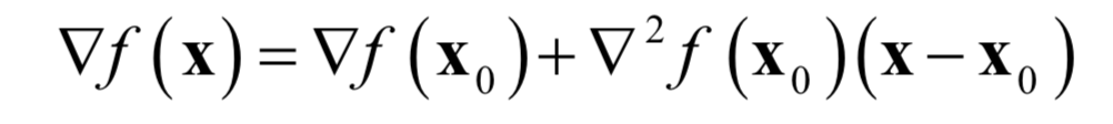
For multivariable functions, perform a second-order Taylor expansion at x0:

Ignoring the second-order and higher terms, the function is approximated as a quadratic function, and taking the gradient of both sides gives the gradient of the function:

where ▽2 f(x0) is the Hessian matrix H. Setting the gradient of the function to 0 yields:

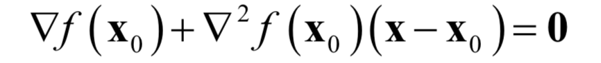
Solving this linear equation can yield:

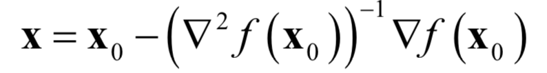
Since higher-order terms were ignored in the Taylor expansion, this solution may not necessarily be the stationary point of the function; it requires repeated iterations using this formula. Starting from the initial point x0, the Hessian matrix and gradient vector of the function at that point are repeatedly calculated, and then the following formula is used for iteration:

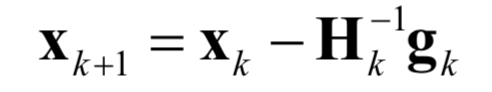
Eventually, it will reach the stationary point of the function. Here, –H–1g is called the Newton direction. The stopping condition for the iteration is when the norm of the gradient approaches 0, or the decrease in function value is less than a specified threshold. For univariate functions, the Hessian matrix is the second derivative, and the gradient vector is the first derivative, with the iteration formula being:

This method will be used in the derivation of XGBoost.

XGBoost is an improvement of the gradient boosting algorithm, using Newton’s method when solving the extreme value of the loss function, expanding the loss function to the second order, and adding a regularization term to the loss function. The objective function during training consists of two parts: the first part is the loss of the gradient boosting algorithm, and the second part is the regularization term. The loss function of XGBoost is defined as:

where n is the number of training samples, l is the loss for a single sample, yi‘ is the predicted value, yi is the true label value of the sample, and Φ is the model parameters. The regularization term defines the complexity of the model.

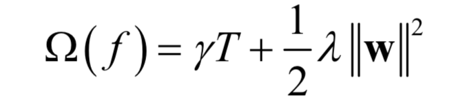
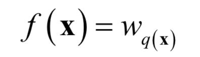
where γ and λ are manually set coefficients, w is the vector formed by the values of all leaf nodes of the decision tree, and T is the number of leaf nodes. The regularization term consists of two components: the number of leaf nodes and the squared norm of the vector of leaf node values, where the first term reflects the complexity of the decision tree structure, and the second term reflects the complexity of the predicted values of the decision tree. Defining q as the mapping from the input vector X to the decision tree leaf node number, that is, determining which leaf node value of the decision tree to use to predict its output value based on the input vector:

where d is the dimensionality of the feature vector. Thus, q defines the structure of the tree, and w defines the output values of the tree. The mapping function of the decision tree can be written as:

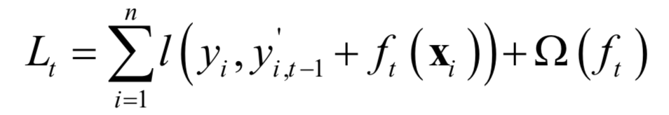
Similar to the gradient boosting algorithm, a strong learner is represented using an additive model. Suppose yi,t‘ is the strong learner’s predicted value for the i-th sample at the t-th iteration, during training, each weak learner function ft is sequentially determined and added to the strong learner’s prediction function, minimizing the following objective function:

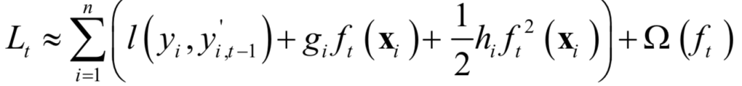
In implementation, a greedy method is used to add ft to the model to minimize the objective function value. Note that here yi is a constant, yi,t-1‘ + f(xi） is the independent variable of the loss function, while yi,t-1‘ is also a constant. For a general loss function, it is not possible to obtain a closed-form solution for the above optimization problem. Newton’s method is used for approximate solving, and the objective function is expanded to the second order Taylor series at the point yi,t-1‘:

The first derivative of the loss function is:

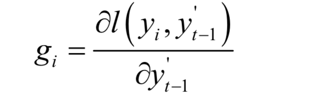
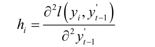
Similar to the gradient boosting algorithm, it treats the predictions of the already trained strong learner for the samples as variables for differentiation; this is a key point to understand, as many readers are confused about whom this derivative is taken with respect to. The second derivative of the loss function is:

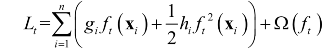
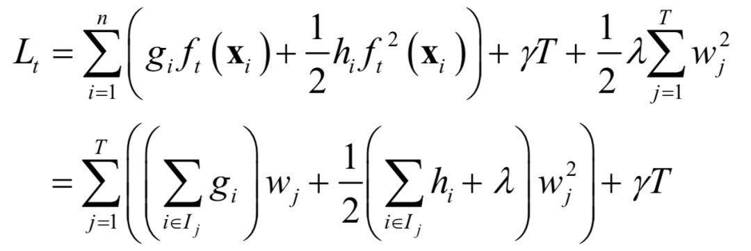
Removing the constant terms unrelated to ft(xi）, the simplified loss function is:

If we define the set:

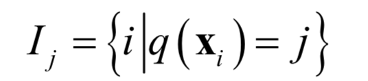
that is, the predicted value belongs to the set of training samples of the j-th leaf node (the set of sample indices). Since each training sample belongs to only one leaf node, the objective function can be split into the sum of loss functions for all leaf nodes:

First, let’s introduce how to determine the values of the leaf nodes. If the structure of the decision tree, that is, q(x), is determined, we can obtain the optimal value of the j-th leaf node using Newton’s method:

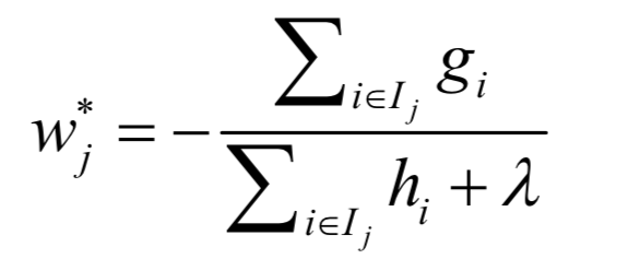
This is the result of taking the derivative of the loss function for a single leaf node with respect to wj and setting the derivative to 0. It has been previously assumed that the loss function for a single sample is convex, thus it must be a minimum. The first derivative of the loss function for a single leaf node with respect to wj is:

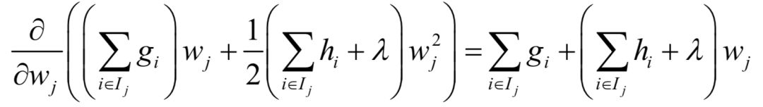
Setting it to 0 yields the above result.

Next, we explain how to determine the structure of the decision tree, that is, how to find the best split. By substituting the optimal solution of wj into the loss function, we obtain a loss function that only contains q:

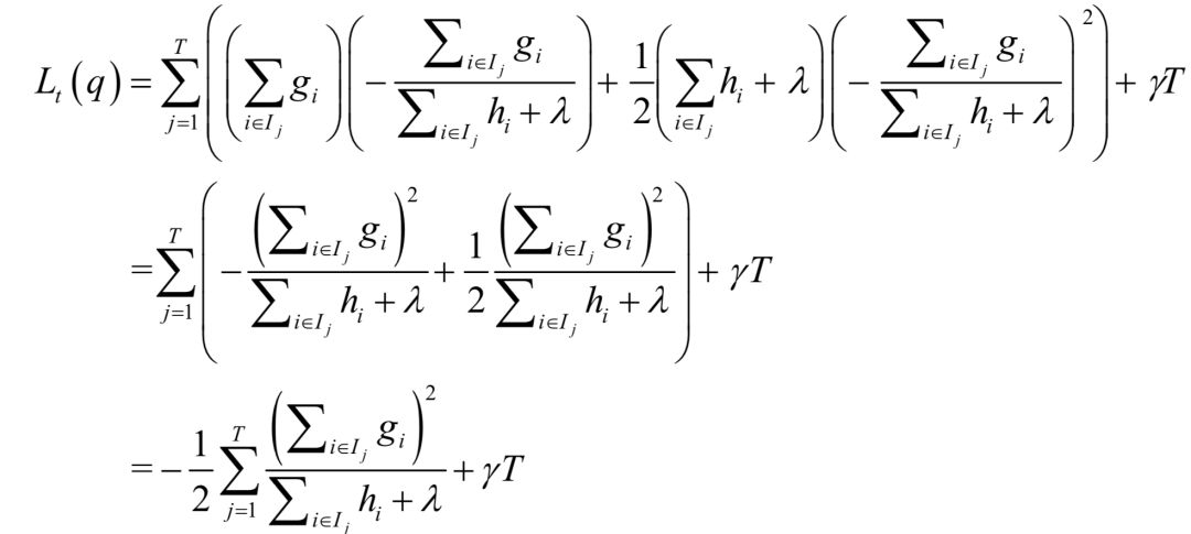
This function can be seen as a measure of the quality of the decision tree structure, and we seek to minimize it, similar to the impurity metrics used when searching for splits in decision trees. Suppose the training sample set before the split is I, and the training sample sets for the left child node and right child node after the split are IL and IR, respectively. After the split, the number of leaf nodes increases by 1, thus the second term of the above objective function changes from γT to γ(T+1), and the difference between the two is γ. Maximizing the decrease in the loss function is equivalent to seeking the maximum of –Lt (q).

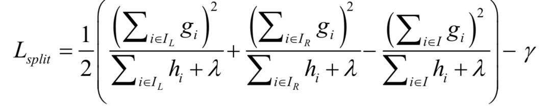
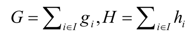
γ is a constant; therefore, the rightmost part of the above equation, –γ, can be ignored. In addition to using different split metrics, the other processes are the same as the standard decision tree training algorithm. In implementation, the summation terms in the above formula are defined as several variables, which are the sums of the first derivatives and second derivatives of all training samples:

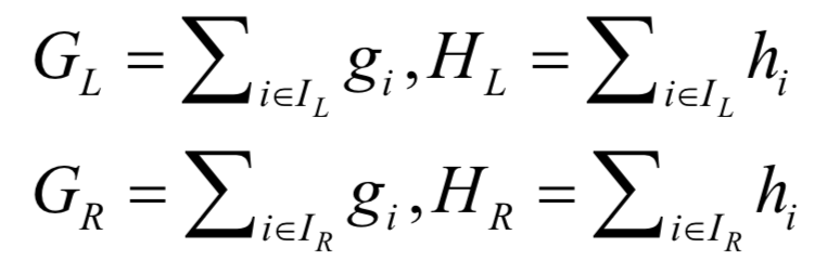
the sums of the first derivatives and second derivatives of the left and right child sample sets:

The algorithm flow for finding the best split is:

Input data I: the current node’s training sample set, with n training samples

Input data d: the dimensionality of the feature vector

Initialize split quality:score ← 0

Calculate the sum of the first derivatives and second derivatives of all samples:G←∑i∈I gi ,H ←∑i∈I hi

Loop over k=1,…,d

Sort all training samples in ascending order based on the k-th feature

Initialize the sum of first derivatives and second derivatives for all training samples in the left child node: GL ←0,HL =0

Loop over j=1,…,n, using the k-th feature component of the j-th sample xjk as the split threshold

Calculate the sum of first derivatives and second derivatives for all samples in the left child node, adding the values of the first derivatives and second derivatives of the samples that have been moved from the right to the left:GL ←GL +gi,HL ←HL +hj

Calculate the sum of first derivatives and second derivatives for all samples in the right child node, which can be quickly calculated based on the total sum and the left child sums:GR ←G–GL,HR ←H–HL

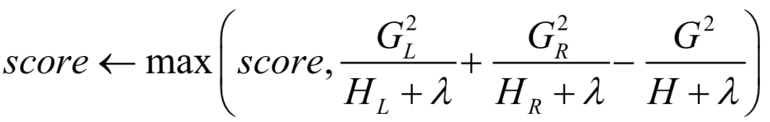
Calculate the maximum value of the split score:

End loop

Return: maximum split quality score and its corresponding split (including selected feature and split threshold)

XGBoost also employs weight shrinking and column sampling techniques to combat overfitting. The weight shrinking method scales the weights of the decision trees trained after each tree, multiplying them by a coefficient η. Weight shrinking reduces the influence of previous decision trees, leaving more space for future decision trees to be generated. The column sampling method is similar to that of random forests; each time the best split is sought, only a portion of randomly selected feature components is considered.

References

[1] Jerome H Friedman. Greedy function approximation: A gradient boosting machine. Annals of Statistics. 2001.
[2] Tianqi Chen, Carlos Guestrin. XGBoost: A Scalable Tree Boosting System. knowledge discovery and data mining. 2016.
[3] Jerome Friedman, Trevor Hastie and Robert Tibshirani. Additive logistic regression: a statistical view of boosting. Annals of Statistics 28(2), 337–407. 2000.
60% off (December 27 – January 31)
2019, the year to start learning!
All products at 60% off (including courses, knowledge base interpretation videos, cloud laboratories)
Purchase method: Log in to [official website] www.sigai.cn to purchase