0. Introduction
This article reviews deep generative models, particularly diffusion models, and how they endow machines with human-like imagination. Diffusion models show great potential in generating realistic samples, overcoming the posterior distribution alignment obstacles in variational autoencoders and alleviating the instability of adversarial objectives in generative adversarial networks.
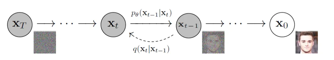
Diffusion models consist of two interconnected processes: a forward process that maps the data distribution to a simple prior distribution and a corresponding reverse process. The forward process resembles simple Brownian motion with time-varying coefficients. Neural networks are trained to estimate score functions using a denoising score matching objective. During the forward diffusion phase, images are gradually contaminated with introduced noise until they become completely random noise. In the reverse process, a series of Markov chains are used to gradually remove predicted noise at each time step, recovering data from Gaussian noise.
However, diffusion models inherently require a more time-consuming iterative process for sampling compared to GANs and VAEs. This is due to the iterative transformation process that utilizes ODE/SDE or Markov processes to convert the prior distribution into a complex data distribution, necessitating numerous function evaluations during the reverse process.
This is attributed to the ability of diffusion models to preserve the semantic structure of data. However, the computational demands of these models are high, requiring very large memory for training, which makes it difficult for most researchers to even attempt this approach. This is because all Markov states need to be kept in memory for prediction, implying that multiple instances of large deep networks are constantly in memory. Additionally, the training time for these methods becomes excessively long (e.g., from days to months) as these models often get trapped in the fine-grained, imperceptible complexities of image data. It is worth noting that this fine-grained image generation is also one of the main advantages of diffusion models, thus using them presents a contradiction.
To address these challenges, researchers have proposed various solutions. For example, advanced ODE/SDE solvers have been proposed to accelerate the sampling process, along with model distillation strategies to achieve this goal. Furthermore, novel forward processes have been introduced to enhance sampling stability or facilitate dimensionality reduction. In recent years, a series of studies have focused on effectively connecting arbitrary distributions using diffusion models. To provide a systematic overview, we categorize these advancements into four main areas: sampling acceleration, diffusion process design, likelihood optimization, and bridging distributions. Additionally, this review will comprehensively examine the various applications of diffusion models across different fields, including computer vision, natural language processing, and healthcare.
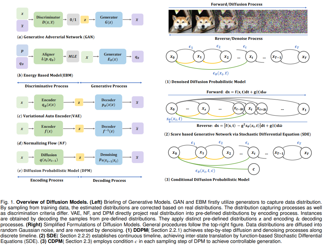
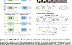
Figure 1. Overview of Diffusion Models. (Left) Introduction to Generative Models. GANs and EBMs first capture the data distribution using a generator. The estimated distribution is corrected based on sampling from the training data according to the true distribution. The capturing processes and discriminative criteria vary. VAEs, NFs, and DPMs project the true distribution directly to a predefined distribution through the encoding process. Instances are obtained by decoding samples from the predefined distribution. They apply different predefined distributions z and encoding-decoding processes. (Right) A simplified form of diffusion models. The general procedure follows the illustration in the upper right. The data distribution is diffused into random Gaussian noise and reversed through the denoising process. (1) DDPM achieves a stepwise diffusion and denoising process along a discrete timeline. (2) SDE establishes a continuous timeline, facilitating state transitions through stochastic differential equations (SDE) based on functions. (3) CDPM utilizes conditional c > at each sampling step in DPM to achieve controllable generation.
1. Algorithm Improvements
Despite the high quality of images generated by diffusion models across various data modalities, their real-world applications still require improvements. Unlike other generative models (such as GANs and VAEs), they necessitate a slow iterative sampling process, and their forward process operates in high-dimensional pixel space. This section highlights four recent developments aimed at enhancing the performance of diffusion models: (1) sampling acceleration techniques (Section 2) to speed up standard ODE/SDE simulations; (2) new forward processes (Section 3) to improve Brownian motion in pixel space; (3) likelihood optimization techniques (Section 4) to enhance the likelihood of diffusion ODEs; (4) bridging distribution techniques (Section 5) that utilize the concepts of diffusion models to connect two different distributions.
2. Sampling Acceleration
Although the image quality generated by diffusion models is high, their practical applications are limited due to slow sampling speed. This section briefly introduces four advanced techniques to improve sampling speed: distillation, training progress optimization, training-free acceleration, and integrating diffusion models with faster generative models.
2.1 ### Forward Diffusion Process
This process serves as a means to transform the data distribution into a predefined distribution, such as a Gaussian distribution. The transformation is represented as: the principle of gradually adding noise to data samples from a certain distribution is called diffusion, transforming them into predefined typically simple distributions, like Gaussian distributions, and then gradually reversing this process to generate data that matches the original data.
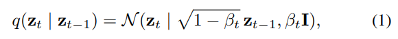
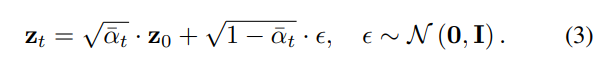
Here, a set of hyperparameters $0 < \beta_{1:T} < 1$ represents the noise variance introduced at each successive step. This diffusion process can be briefly expressed through a single-step equation:

Where $\alpha_t = 1 – \beta_t$ and $\bar{\alpha}_t = \prod_{i=1}^t \alpha_i$, as detailed by Sohl-Dickstein et al. [15]. Therefore, bypassing the need to consider intermediate time steps, $z_t$ can be directly sampled as follows:
2.2 Reverse Diffusion Process
The primary goal here is to learn the inverse process of the forward diffusion process, aiming to generate a distribution closely aligned with the original unaltered data sample $z_0$. In the context of image editing, $z_0$ represents the edited image. In practice, this is achieved by learning a parameterized version of $p$ using the UNet architecture. Considering that the forward diffusion process is approximated as $q(z_T) \approx N(0, I)$, the learnable transformation formula is expressed as:

Here, the functions $µ_θ$ and $Σ_θ$ are learnable parameters. Furthermore, for the conditional formula $p_θ (z_{t−1} | z_t, c)$, it is conditioned on an external variable $c$ (in image editing, $c$ can be the source image), transforming the model to $µ_θ(z_t, c, \bar{α}_t)$ and $Σ_θ(z_t, c, \bar{α}_t)$.
2.3 Optimization
The optimization strategy guiding reverse diffusion learning of the forward process involves minimizing the Kullback-Leibler (KL) divergence between the joint distributions of the forward and reverse sequences. These are mathematically defined as:
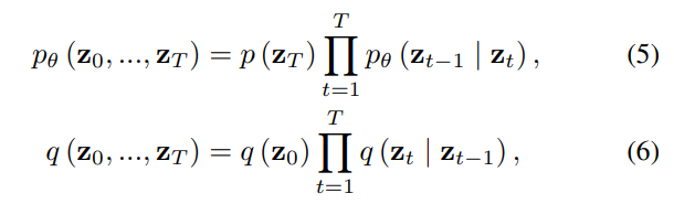
Leading to minimization:
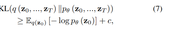
This is detailed in the work of Ho et al. [16], where the constant $c$ is irrelevant for optimizing $θ$. The KL divergence in Equation 7 represents the variational upper bound of the log likelihood of the data $(log p_θ(z_0))$. This KL divergence serves as a loss and is minimized in denoising diffusion probabilistic models (DDPMs). In fact, Ho et al. [16] adopted a reweighted version of this loss as a simpler denoising loss:
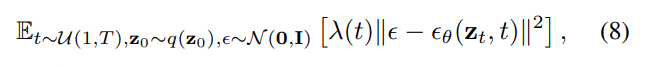
Where $λ(t) > 0$ represents a weight function, $z_t$ is obtained through Equation 3, and $ϵ_θ$ denotes a network aimed at predicting noise $ϵ$ based on $z_t$ and $t$.
2.4 DDIM Sampling and Inversion
When handling real images $z_0$, popular editing methods [84], [85] initially use specific inversion schemes to invert this $z_0$ into the corresponding $z_T$. Subsequently, sampling starts from this $z_T$, employing some editing strategies to produce the edited result $ ilde{z}_0$. Ideally, directly sampling from $z_T$ without any edits should yield a $ ilde{z}_0$ that closely resembles $z_0$. A significant deviation of $ ilde{z}_0$ from $z_0$, termed reconstruction failure, indicates that the edited image fails to maintain the integrity of the unchanged areas in $z_0$. Therefore, it is crucial to utilize an inversion method that ensures $ ilde{z}_0 ≈ z_0$.
The DDIM sampling equation [18] is:
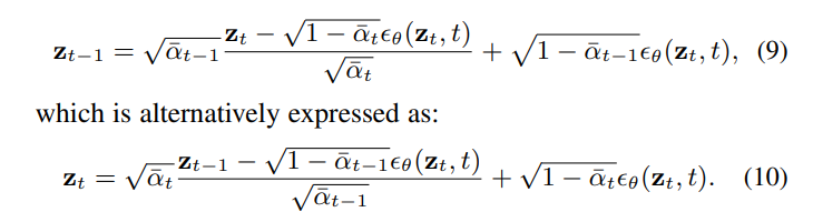
The above (9) can be replaced by (10).
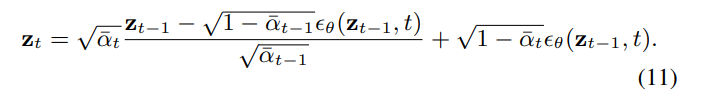
While Equation 10 appears to provide an ideal inversion from $z_{t−1}$ to $z_t$, the problem arises with the unknown nature of $z_t$, which is also used as input for the network $ϵ_θ(z_t, t)$. To address this issue, DDIM inversion [18] operates under the assumption that $z_{t−1} ≈ z_t$, replacing $z_t$ on the right side of Equation 10 with $z_{t−1}$, leading to the following approximation:
2.5 Text Conditioning and Classifier-Free Guidance
Text-conditioned diffusion models aim to synthesize results starting from random noise $z_T$, guided by text prompts $P$. In the inference of the sampling process, a noise estimation network $ϵ_θ(z_t, t, C)$ is used to predict noise $ϵ$, where $C = ψ(P)$ represents the text embedding. This process systematically removes noise from $z_t$ across $T$ steps until the final result $z_0$ is obtained.
In the field of text-conditioned image generation, ensuring substantial text influence and control over the generated output is crucial. To this end, Ho et al. [86] introduced the concept of classifier-free guidance, a technique that combines conditional and unconditional predictions. More specifically, let $∅ = ψ(“”)1$ represent an empty text embedding. When combined with a guidance scale $w$, classifier-free guidance predictions are formalized as:

In this formula, $ϵθ(zt, t, C, ∅)$ replaces $ϵθ(zt, t)$ in the sampling equation 9. The value of $w$ typically ranges from [1, 7.5], as suggested in [26], [27], determining the extent of text control. Higher values of $w$ are associated with stronger text-driven influences during the generation process.
3. Related Tasks
3.1 Conditional Image Generation
While we primarily focus on diffusion models in image editing, it is important to acknowledge related areas, such as conditional image generation. Unlike image editing, which involves modifying certain parts of existing images, conditional image generation entails creating new images from scratch, guided by specified conditions. Early works [31], [32], [87]–[90] often involved class-conditional image generation, typically incorporating class-induced gradients into the sampling process through additional pre-trained classifiers. However, Ho et al. [86] introduced classifier-free guidance, which does not rely on external classifiers and allows for more diverse conditions, such as text, to serve as guidance.
Text-to-Image (T2I) Generation. GLIDE [34] is the first work to directly use text to guide image generation at the high-dimensional pixel level, replacing labels in class-conditional diffusion models. Similarly, Imagen [27] employs a cascading framework to generate high-resolution images more efficiently in pixel space. Different research lines project images into a low-dimensional space and then apply diffusion models in this latent space. Representative works include Stable Diffusion (SD) [26], VQ-Diffusion [91], and DALL-E 2 [25]. Following these pioneering studies, a considerable amount of work [37], [92]–[97] has been proposed, advancing this field over the past two years.
Additional Conditions. In addition to text, more specific conditions have also been employed to achieve higher fidelity and more precise control in image synthesis. GLIGEN [98] inserts a gated self-attention layer between the original self-attention and cross-attention layers in each block to generate condition-based images based on bounding boxes. Make-A-Scene [99] and SpaText [100] guide the generation process using segmentation masks. In addition to segmentation maps, ControlNet [101] can incorporate other types of inputs, such as depth maps, normal maps, canny edges, poses, and sketches as conditions. Other methods such as UniControlNet [102], UniControl [103], Composer [104], and T2I-Adapter [105] integrate diverse conditional inputs and add additional layers to enhance the generation process under these conditional controls.
Customized Image Generation. A task closely related to conditional image generation and image editing is creating personalized images. This task focuses on generating images that maintain a certain identity, usually guided by several reference images of the same subject. Two early methods for addressing this customized generation with a few images are text inversion [106] and DreamBooth [107]. Specifically, text inversion learns a unique identifying word to represent a new subject and incorporates this word into the dictionary of the text encoder. On the other hand, DreamBooth fine-tunes the entire Imagen [27] model using a few reference images, binding a new rare word to a specific subject. To effectively combine multiple new concepts, CustomDiffusion [108] only optimizes the cross-attention parameters in Stable Diffusion [26], jointly training to represent new concepts and enable multi-concept combinations.
3.2 Image Restoration and Enhancement
Image restoration (IR) is a key task in low-level vision aimed at improving the quality of images contaminated by various degradations. Recent advances in diffusion models have prompted researchers to explore their potential in image restoration. Pioneering attempts to integrate diffusion models into this task have surpassed previous GAN-based methods.
Using Input Images as Conditions. Generative models have significantly facilitated the development of various image restoration tasks, such as super-resolution (SR) and deblurring [12], [13], [29], [118], [119]. Through a repeated refinement process, Super-Resolution (SR3) [57] utilizes DDPM for conditional image generation via random iterative denoising. Cascading diffusion models [31] sequentially adopt multiple diffusion models, each generating higher resolution images. SRDiff [118] closely realizes the concept of SR3. The main difference between SRDiff and SR3 is that SR3 directly predicts the target image, while SRDiff predicts the difference between the input and output images.
Restoration in Non-Spatial Domains. Some IR methods based on diffusion models focus on other spaces. For instance, Refusion [63], [120] uses average regression image restoration (IR)-SDE to convert target images into their degraded counterparts. They utilize autoencoders to compress input images into their latent representations and access multi-scale details through skip connections. Chen et al. [121] adopt a similar approach, proposing a two-stage strategy termed hierarchical integrated diffusion models. The transition from spatial domain to wavelet domain is lossless, providing significant advantages. For example, WaveDM [67] modifies the low-frequency bands, while WSGM [122] or ResDiff [60] conditions high-frequency bands relative to low-resolution images. BDCE [123] designs a guided diffusion model in deep curve space for enhancing low-light high-resolution images.
Using T2I Information. Integrating T2I information has proven beneficial as it allows the use of pre-trained T2I models. These models can be fine-tuned by adding specific layers or encoders tailored for IR tasks. Wang et al. put this concept into practice by creating StableSR [124]. The core of StableSR is a time-aware encoder trained alongside a frozen stable diffusion model [26]. This setup seamlessly integrates trainable spatial feature transformation layers, enabling conditioning based on input images. DiffBIR [125] employs a pre-trained T2I diffusion model for blind image restoration, featuring a two-stage pipeline and a controllable module. CoSeR [126] introduces cognitive super-resolution, merging image appearance with language understanding. SUPIR [127] utilizes generative priors, model scaling, and a dataset of 20 million images, guiding advanced restoration through text prompts, including negative quality prompts and restoration-guided sampling methods.
Projection-Based Methods. These methods aim to extract inherent structures or textures from input images to complement the images generated at each step and ensure data consistency. ILVR [65] ensures data consistency by projecting the low-frequency information of the input image onto the output image, establishing improved conditions. To address this issue and enhance data consistency, some recent works [70], [71], [128] have taken different approaches, aiming to estimate posterior distributions using Bayesian theorem.
Decomposition-Based Methods. These methods treat IR tasks as linear inverse problems. The Denoising Diffusion Restoration Model (DDRM) [66] utilizes a pre-trained denoising diffusion generative model to tackle linear inverse problems, demonstrating versatility across various noise levels in super-resolution, deblurring, restoration, and colorization. The Denoising Diffusion Zero-Point Model (DDNM) [68] represents another decomposition-based zero-order attempt applicable to a wide range of linear IR problems beyond super-resolution, such as colorization, restoration, and deblurring. It effectively addresses various IR challenges using range-zero space decomposition methods [129], [130].
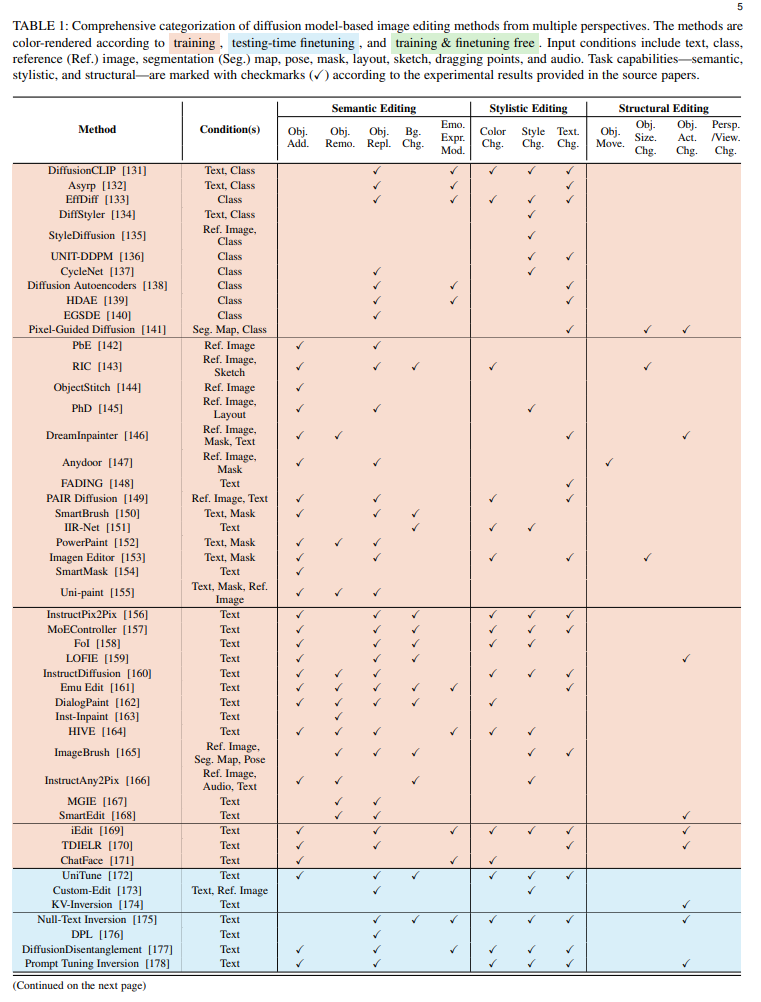
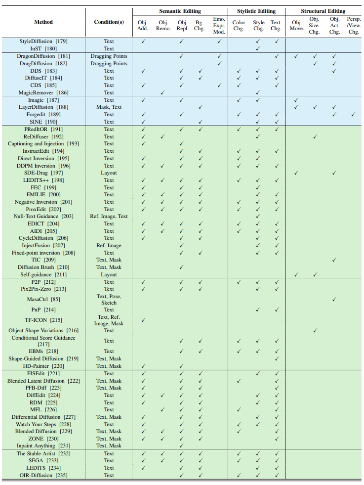
Table 1: A comprehensive categorization of image editing methods based on diffusion models from multiple perspectives. Color rendering is performed based on training, fine-tuning during testing, and methods without training or fine-tuning. Input conditions include text, class, reference (Ref.) images, segmentation (Seg.) maps, poses, masks, layouts, sketches, drag points, and audio. Task capabilities—semantic, style, and structure—are marked with checkmarks (✓) based on experimental results provided in the source papers.
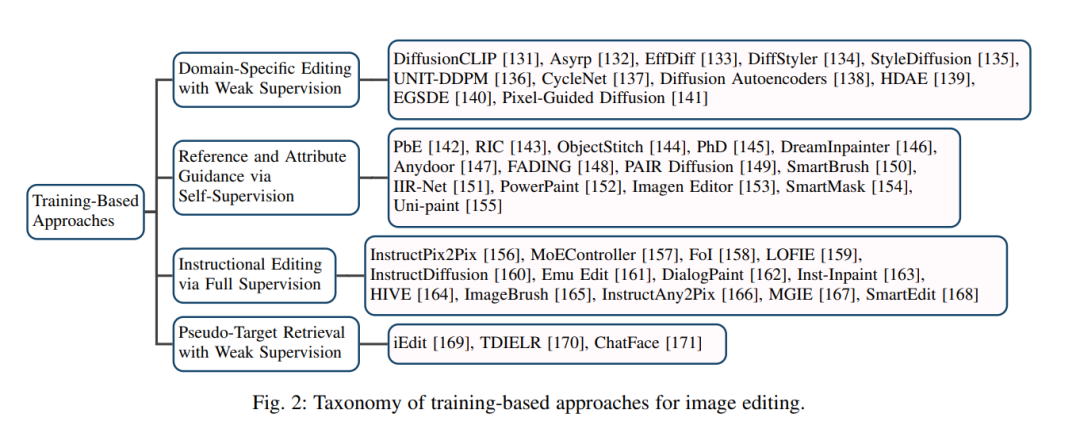
Figure 2: Classification of training-based image editing methods.
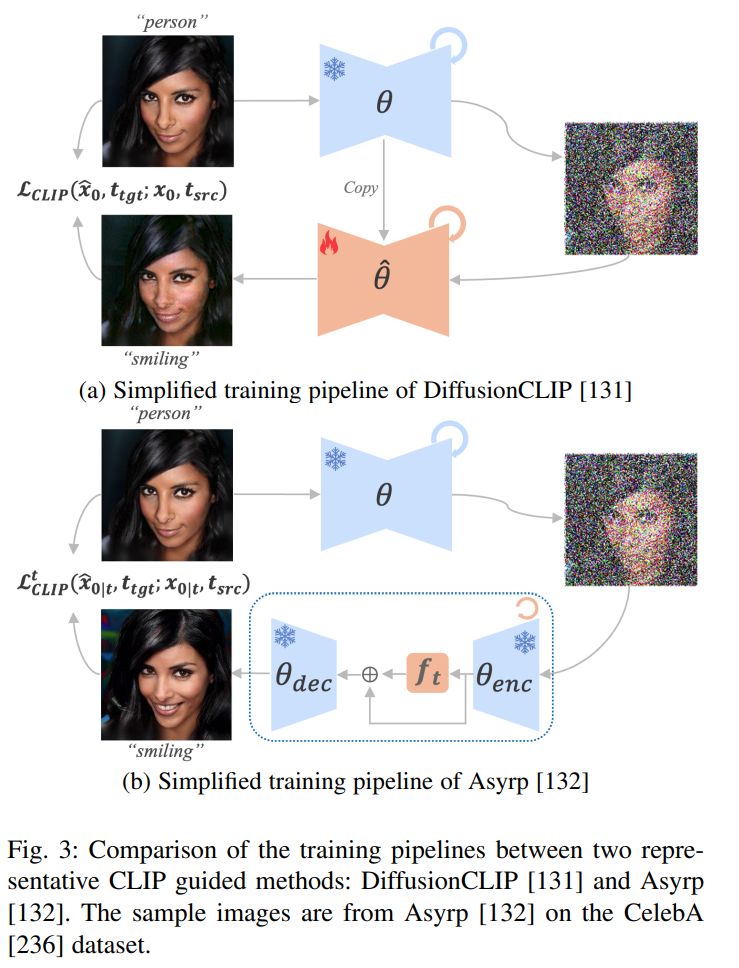
Figure 3: Comparison of training processes between two representative CLIP-guided methods, DiffusionCLIP [131] and Asyrp [132]. Sample images are sourced from the application of Asyrp [132] on the CelebA [236] dataset.

Figure 4: A general framework for instructive image editing methods. Example images are sourced from InstructPix2Pix [156], InstructAny2Pix [166], and MagicBrush [249].
4. Reference Links
https://mp.weixin.qq.com/s/MFbCt0XfOf9fV0YbdkmR6g