Author: yyHaker
Source: https://zhuanlan.zhihu.com/p/136521625


This article is about 5900 words long and is recommended to be read in 10 minutes. This article will provide a simple summary from a more intuitive perspective of the currently popular classic GNN networks, including GCN, GraphSAGE, GAT, GAE, and graph pooling strategies such as DiffPool.
In recent years, the enthusiasm for research on Graph Neural Networks (GNN) in the field of deep learning has been growing. GNN has become a hot topic of research at major deep learning conferences. The excellent ability of GNN to handle unstructured data has led to breakthroughs in network data analysis, recommendation systems, physical modeling, natural language processing, and combinatorial optimization problems on graphs.There are many good reviews of Graph Neural Networks [1][2][3] that can be referenced, and more papers can be found in the GNN paper list compiled by Tsinghua University [4]. This article will provide a simple summary from a more intuitive perspective of the currently popular classic GNN networks, including GCN, GraphSAGE, GAT, GAE, and graph pooling strategies such as DiffPool.
1. Why Do We Need Graph Neural Networks?
With the development of machine learning and deep learning, significant breakthroughs have been made in speech, image, and natural language processing. However, speech, images, and texts are all simple sequence or grid data, which are very structured data types that deep learning excels at handling (Figure 1).
Figure 1However, in the real world, not everything can be represented as a sequence or a grid, such as social networks, knowledge graphs, complex file systems, etc. (Figure 2), which means that many things are unstructured.Figure 2Compared to simple text and images, this type of unstructured network data is very complex, and the challenges in processing it include:
The size of the graph is arbitrary, and the graph’s topology is complex, lacking spatial locality like images;
Graphs do not have a fixed node order, or there is no reference node;
Graphs are often dynamic and contain multimodal features.
So how should we model this type of data? Can deep learning be extended to model this type of data? These questions have prompted the emergence and development of Graph Neural Networks.
2. What Are Graph Neural Networks Like?
Compared to the most basic network structure of neural networks, the fully connected layer (MLP), where the feature matrix is multiplied by the weight matrix, Graph Neural Networks add an adjacency matrix. The calculation is quite simple, involving the multiplication of three matrices followed by a non-linear transformation (Figure 3).Figure 3Thus, a common application pattern of Graph Neural Networks is as follows (Figure 4), where the input is a graph, and after multiple layers of graph convolution and various operations, along with activation functions, the representations of each node are obtained for tasks such as node classification, link prediction, and graph and subgraph generation.Figure 4The above provides a relatively simple and intuitive understanding of Graph Neural Networks, but the underlying principles and logic are quite complex, which will be discussed further later. Next, we will introduce the development of Graph Neural Networks through several classic GNN models.
3. Several Classic Models of Graph Neural Networks and Their Development
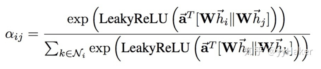
1. Graph Convolution Networks (GCN) [5]GCN can be considered the “foundational work” of Graph Neural Networks, as it was the first to apply the convolution operation from image processing to the processing of graph-structured data and provided a specific derivation involving complex spectral graph theory. The detailed derivation can be referenced [6][7]. The derivation process is quite complex, but the final result is very simple (Figure 5).Figure 5Let’s take a look at this equation. Oh my, isn’t this just aggregating the features of neighboring nodes and then performing a linear transformation? That’s right, it is indeed. Additionally, to enable GCN to capture information from K-hop neighboring nodes, the authors stack multiple layers of GCN layers, such as stacking K layers:The above equation can also be expressed in matrix form as follows:Where is the normalized adjacency matrix, and represents a linear transformation of all nodes’ embeddings in the layer. The left multiplication by the adjacency matrix indicates that for each node, its feature representation is the sum of its neighbors’ features (Note that replacing with a matrix corresponds to the three matrices’ multiplication mentioned in Figure 3).So how effective is GCN? The authors applied GCN to node classification tasks and conducted experiments on datasets such as Citeseer, Cora, Pubmed, and NELL. The improvement compared to traditional methods is significant, likely due to GCN’s ability to encode graph structural information and learn better node representations.Figure 6Of course, the drawbacks of GCN are also quite evident. First, GCN requires the entire graph to be loaded into memory, which can be very memory-intensive and may not handle large graphs. Second, GCN needs to know the entire graph’s structural information (including the nodes to be predicted) during training, which can be challenging in some real-world tasks (for example, using a model trained today to predict data for tomorrow, when tomorrow’s nodes are not available).2. Graph Sample and Aggregate (GraphSAGE) [8]To address the two drawbacks of GCN, GraphSAGE was proposed. Before introducing GraphSAGE, let’s first explain Inductive learning and Transductive learning. Noticing the difference between graph data and other types of data, each node in graph data can utilize the information of other nodes through edge relationships.This leads to a problem: GCN inputs the entire graph, and when training nodes collect information from neighboring nodes, it uses samples from the test and validation sets, which we call Transductive learning. However, most of the machine learning problems we deal with are Inductive learning, as we intentionally split the sample set into training/validation/testing, and during training, only training samples are used. This is beneficial for graphs as it allows handling newly arrived nodes and generating embeddings for unknown nodes using known nodes’ information. GraphSAGE does just that.GraphSAGE is an Inductive Learning framework. In its implementation, during training, it only retains edges from training samples to training samples, and it includes two major steps: Sample and Aggregate. Sample refers to how to sample the number of neighbors, and Aggregate refers to how to aggregate the embeddings of neighboring nodes to update its own embedding information after obtaining them. The following diagram illustrates the learning process of GraphSAGE.Figure 7 Step one: Sample neighbors;Step two: The sampled neighbors’ embeddings are passed to the node, and an aggregation function is used to aggregate this neighbor information to update the node’s embedding;Step three: Based on the updated embedding, predict the node’s label;Next, we will explain in detail how a trained GraphSAGE generates embeddings for a new node (i.e., a forward propagation process), as shown in the algorithm diagram:First, (line 1) the algorithm initializes the feature vectors of all nodes in the input graph, (line 3) for each node , after obtaining its sampled neighboring nodes, (line 4) it aggregates the information of neighboring nodes using the aggregation function, (line 5) and updates its own embedding representation by combining its own embedding through a non-linear transformation.Note that in the algorithm, refers to the number of aggregators, which also indicates the number of weight matrices and the number of layers in the network. This is because in each layer of the network, the aggregator and weight matrices are shared. The number of network layers can be understood as the maximum hops to access neighbors. For example, in Figure 7, the red node’s update obtains information from its first and second-hop neighbors, so the number of network layers is 2. To update the red node, we first in the first layer (k=1), aggregate the blue node’s information to the red node, and aggregate the green node’s information to the blue node. In the second layer (k=2), the red node’s embedding is updated again, but this time it uses the updated blue node’s embedding, ensuring that the updated embedding of the red node includes information from both the blue and green nodes, i.e., two-hop information.To make it clearer, we will expand on the process of updating a certain node, as shown in Figure 8, which illustrates the processes of updating node A and node B. It can be seen that the process of updating different nodes shares the aggregator and weight matrices in each layer of the network.Figure 8So how does GraphSAGE perform sampling? GraphSAGE uses a fixed-length sampling method. Specifically, it defines the required number of neighbors , and then uses resampling with replacement/negative sampling methods to achieve . This ensures that each node (after sampling) has a consistent number of neighbors, which is necessary to concatenate multiple nodes and their neighbors into a tensor for batch training on a GPU.What aggregators does GraphSAGE use? There are three main ones:It is worth noting that the Mean Aggregator and GCN’s approach are basically the same (GCN actually sums them).So far, we have completed the explanation of the entire model architecture. How does GraphSAGE learn the parameters of the aggregators and weight matrices ? In the supervised case, the cross-entropy between each node’s predicted label and true label can be used as the loss function. In the unsupervised case, it can be assumed that the embeddings of neighboring nodes are as close as possible, thus designing the following loss function:So how does GraphSAGE perform in actual experiments? The authors provided unsupervised and fully supervised results on the Citation, Reddit, and PPI datasets, showing a significant improvement over traditional methods.This concludes the introduction to GraphSAGE. Let’s summarize some of its advantages:(1) By utilizing a sampling mechanism, it effectively addresses the issue of GCN needing to know the entire graph’s information, overcoming the memory and GPU limitations during GCN training, and can obtain representations even for unknown new nodes;(2) The parameters of the aggregator and weight matrices are shared among all nodes;(3) The number of model parameters is independent of the number of nodes in the graph, which allows GraphSAGE to handle larger graphs;(4) It can handle both supervised and unsupervised tasks.(I love ideas that solve problems simply and effectively!!!)Of course, GraphSAGE also has some drawbacks. Given that each node has so many neighbors, GraphSAGE’s sampling does not consider the differing importance of different neighboring nodes, and the importance of neighboring nodes during aggregation may differ from that of the current node.3. Graph Attention Networks (GAT) [9]To address the issue of GNN not considering the varying importance of neighboring nodes during aggregation, GAT borrows ideas from Transformers and introduces a masked self-attention mechanism. When calculating the representations of each node in the graph, different weights are assigned based on the features of neighboring nodes.Specifically, for the input graph, a graph attention layer is shown in Figure 9:
Figure 9
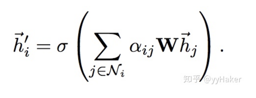
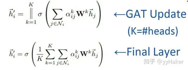
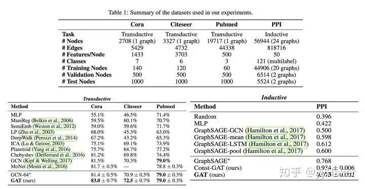
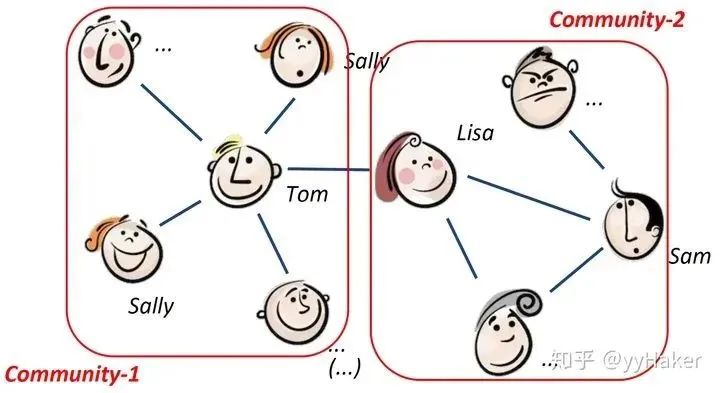
In which employs a single-layer feedforward neural network for implementation, and the calculation process is as follows (note that the weight matrix is shared among all nodes):After calculating the attention, a new representation of a node aggregating its neighboring nodes’ information can be obtained, with the calculation process as follows:To enhance the model’s fitting ability, a multi-head self-attention mechanism is introduced, which simultaneously uses multiple to compute self-attention and then merges (either concatenates or sums) the computed results:Additionally, due to the structural characteristics of GAT, it does not require using a pre-constructed graph, making GAT suitable for both Transductive Learning and Inductive Learning.How effective is GAT? The authors conducted experiments on three Transductive Learning tasks and one Inductive Learning task, with the results as follows:In both Transductive Learning and Inductive Learning tasks, GAT outperformed traditional methods.This concludes the introduction to GAT. Let’s summarize some of its advantages:(1) Training GCN does not require knowledge of the entire graph structure, only the neighboring nodes of each node are needed;(2) It has a fast computation speed and can perform parallel calculations on different nodes;(3) It can be used for both Transductive Learning and Inductive Learning, allowing it to handle unseen graph structures.(Once again, a simple idea that solves a problem effectively!!!)So far, we have introduced the most classic models in GNN: GCN, GraphSAGE, and GAT. Next, we will introduce some popular GNN models and methods for specific task categories.4. Unsupervised Node Representation LearningDue to the high cost of labeled data, if we can effectively learn node representations using unsupervised methods, it will have enormous value and significance, such as finding communities with similar interests and discovering interesting structures in large-scale graphs, etc.Figure 10Among these, classic models include GraphSAGE and Graph Auto-Encoder (GAE), etc. GraphSAGE is a very good unsupervised representation learning method, which has been introduced earlier, so it will not be repeated here. Next, we will detail the latter two.
Graph Auto-Encoder (GAE) [10]
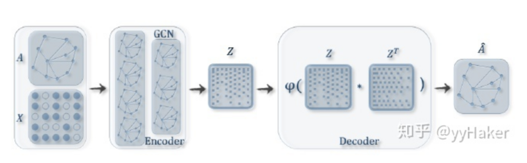
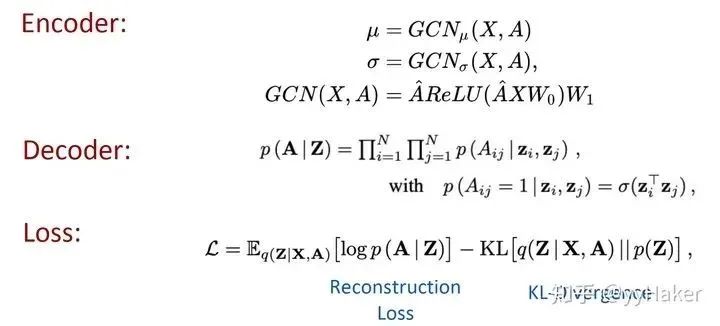
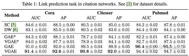
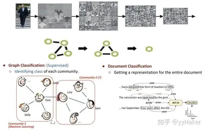
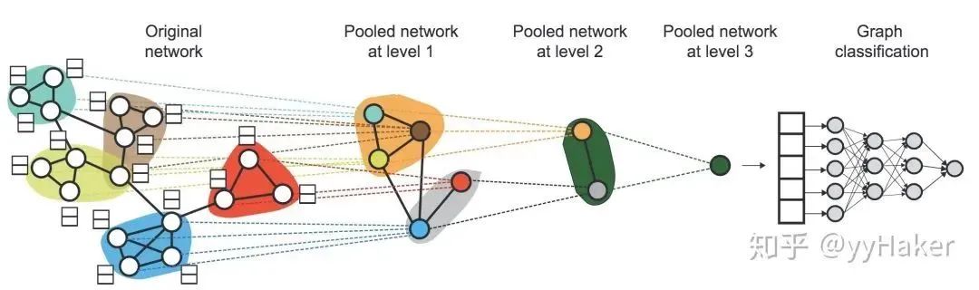
Before introducing Graph Auto-Encoder, it is necessary to understand Auto-Encoders and Variational Auto-Encoders, which can be referenced [11], and will not be elaborated here.Once you understand Auto-Encoders, understanding Variational Graph Auto-Encoders becomes much easier. As shown in Figure 11, the input graph’s adjacency matrix and node feature matrix are used to learn the mean μ and variance σ of the low-dimensional vector representations of nodes through an encoder (graph convolution network), and then the decoder (link prediction) generates the graph.Figure 11The encoder uses a simple two-layer GCN network, while the decoder calculates the probability of an edge existing between two points to reconstruct the graph. The loss function includes the distance metric between the generated graph and the original graph, as well as the KL divergence between the node representation vector distribution and the normal distribution. The specific formula is shown in Figure 12:Figure 12Additionally, for comparison, the authors proposed the Graph Auto-Encoder, which is simpler than the Variational Graph Auto-Encoder. The encoder is two-layer GCN, and the loss only contains Reconstruction Loss.How effective are the two types of graph auto-encoders? The authors conducted link prediction tasks on the Cora, Citeseer, and Pubmed datasets, with the experimental results as follows. The Graph Auto-Encoder (GAE) and Variational Graph Auto-Encoder (VGAE) generally outperform traditional methods, and the Variational Graph Auto-Encoder performs better; however, GAE achieved the best results on Pubmed. This may be because the Pubmed network is larger, and the VGAE model is more complex than GAE, making it harder to tune parameters.5. Graph PoolingGraph pooling is a popular operation in GNN, aimed at obtaining a representation of an entire graph, primarily used for graph-level classification tasks, such as supervised graph classification and document classification.Figure 13There are many methods for graph pooling, such as simple max pooling and mean pooling; however, these two pooling methods are inefficient and ignore the order information of nodes. Here, we introduce a method: Differentiable Pooling (DiffPool).1. DiffPool [12]In graph-level tasks, many current methods perform global pooling on all node embeddings, ignoring any hierarchical structures that may exist in the graph. This is particularly problematic for graph classification tasks, as the goal is to predict the label of the entire graph. To address this issue, a team from Stanford University proposed a differentiable pooling operation module for graph classification—DiffPool, which can generate hierarchical representations of graphs and can be integrated with various graph neural networks in an end-to-end manner.The core idea of DiffPool is to hierarchically aggregate graph nodes through a differentiable pooling operation module. Specifically, this differentiable pooling operation module is based on the node embeddings generated by the previous layer of GNN and a distribution matrix, which allocates clusters to the next layer in an end-to-end manner, then inputs these clusters into the next layer of GNN, thereby achieving the idea of stacking multiple GNN layers in a hierarchical manner (Figure 14).Figure 14So how are the node embeddings and distribution matrices computed? After computing, how are they allocated to the next layer? This involves two parts: the learning of the distribution matrix and the pooling distribution matrix.
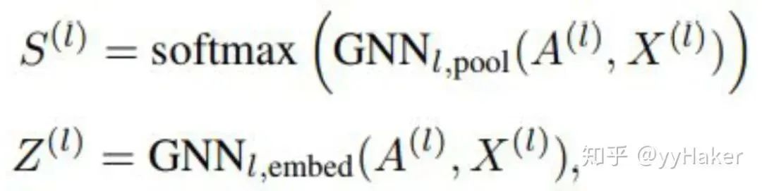
Learning the Distribution Matrix
Two separate GNNs are used to generate the distribution matrix and new embeddings for each cluster node, where both GNNs use the cluster node feature matrix and the coarsened adjacency matrix as inputs:
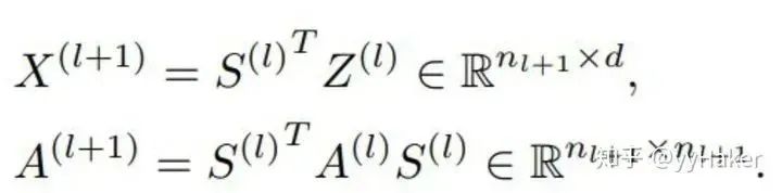
Pooling Distribution Matrix
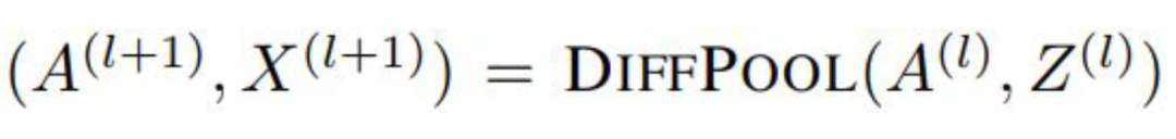
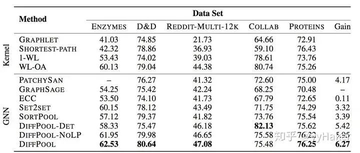
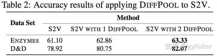
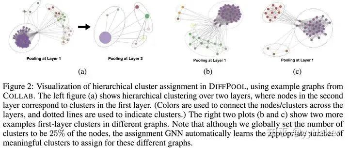
After obtaining the distribution matrix and new embeddings for each cluster node, the DiffPool layer generates a new coarsened adjacency matrix and new embedding matrix for each node/cluster in the graph based on the distribution matrix:Overall, each layer of DiffPool actually updates the embeddings of each cluster node and the feature matrix of the cluster nodes, as shown in the following formula:This concludes the basic idea of DiffPool. How effective is it? The authors conducted experiments on multiple benchmark datasets for graph classification, such as protein datasets (ENZYMES, PROTEINS, D&D), social network datasets (REDDIT-MULTI-12K), and scientific collaboration datasets (COLLAB), with the experimental results as follows:Among them, GraphSAGE uses global average pooling; DiffPool-DET is a variant of DiffPool that uses a deterministic graph clustering algorithm to generate the distribution matrix; DiffPool-NOLP is a variant of DiffPool that removes the link prediction target part. Overall, the DiffPool method achieves the highest average performance among all pooling methods in GNN.To better demonstrate the effectiveness of DiffPool for graph classification, the paper also utilized other GNN architectures (Structure2Vec (s2v)) and constructed two variants for comparative experiments, as shown in the following table:It can be seen that DiffPool significantly improved the performance of S2V on the ENZYMES and D&D datasets.Moreover, DiffPool can automatically learn the appropriate number of clusters.In conclusion, let’s summarize the advantages of DiffPool:(1) It can learn hierarchical pooling strategies;(2) It can learn hierarchical representations of graphs;(3) It can be integrated with various graph neural networks in an end-to-end manner.However, it should be noted that DiffPool also has its limitations; the distribution matrix requires a large amount of space for storage, with spatial complexity of , where is the number of pooling layers, making it unable to handle very large graphs.
References
[1] Graph Neural Networks: A Review of Methods and Applications. arxiv 2018 https://arxiv.org/pdf/1812.08434.pdf[2] A Comprehensive Survey on Graph Neural Networks. arxiv 2019. https://arxiv.org/pdf/1901.00596.pdf[3] Deep Learning on Graphs: A Survey. arxiv 2018 https://arxiv.org/pdf/1812.04202.pdf[4] GNNpapers https://github.com/thunlp/GNNPapers/blob/master/README.md[5] Semi-Supervised Classification with Graph Convolutional Networks(ICLR2017) https://arxiv.org/pdf/1609.02907[6] How to Understand Graph Convolutional Network (GCN)? https://www.zhihu.com/question/54504471[7] GNN Series: The Foundational Work of Graph Neural Networks CGN Model https://mp.weixin.qq.com/s/jBQOgP-I4FQT1EU8y72ICA[8] Inductive Representation Learning on Large Graphs(2017NIPS) https://cs.stanford.edu/people/jure/pubs/graphsage-nips17.pdf[9] Graph Attention Networks(ICLR2018) https://arxiv.org/pdf/1710.10903[10] Variational Graph Auto-Encoders (NIPS2016) https://arxiv.org/pdf/1611.07308[11] VGAE (Variational graph auto-encoders)Detailed Paper Analysis https://zhuanlan.zhihu.com/p/78340397[12] Hierarchical Graph Representation Learning with Differentiable Pooling(NIPS2018) https://arxiv.org/pdf/1806.08
Highlights of This Article
1. The drawbacks of GCN are quite evident:
First, GCN requires the entire graph to be loaded into memory, which can be very memory-intensive and may not handle large graphs;
Second, GCN needs to know the entire graph’s structural information (including the nodes to be predicted).
2. Advantages of GraphSAGE:
(1) By utilizing a sampling mechanism, it effectively addresses the issue of GCN needing to know the entire graph’s information, overcoming the memory and GPU limitations during training, and can obtain representations even for unknown new nodes;
(2) The parameters of the aggregator and weight matrices are shared among all nodes;
(3) The number of model parameters is independent of the number of nodes in the graph, which allows GraphSAGE to handle larger graphs; (4) It can handle both supervised and unsupervised tasks.
3. Advantages of GAT:
(1) Training GCN does not require knowledge of the entire graph structure, only the neighboring nodes of each node are needed;
(2) It has a fast computation speed and can perform parallel calculations on different nodes;
(3) It can be used for both Transductive Learning and Inductive Learning, allowing it to handle unseen graph structures.
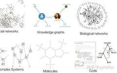
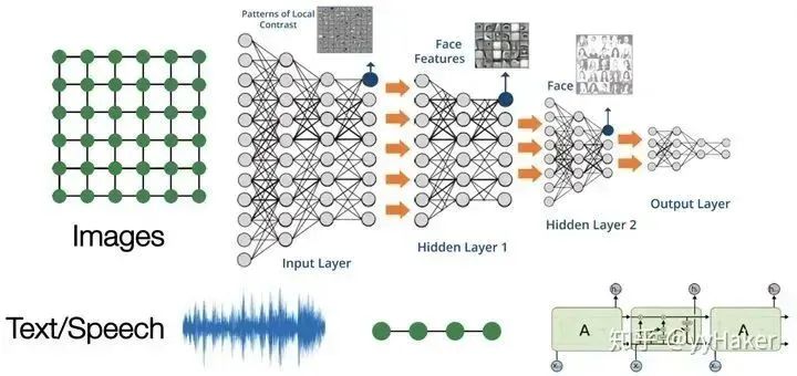
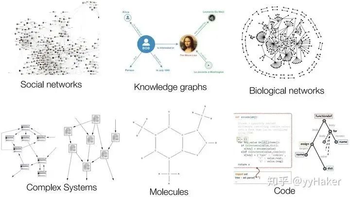
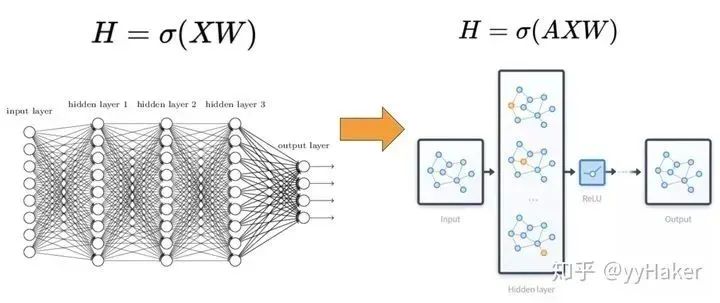
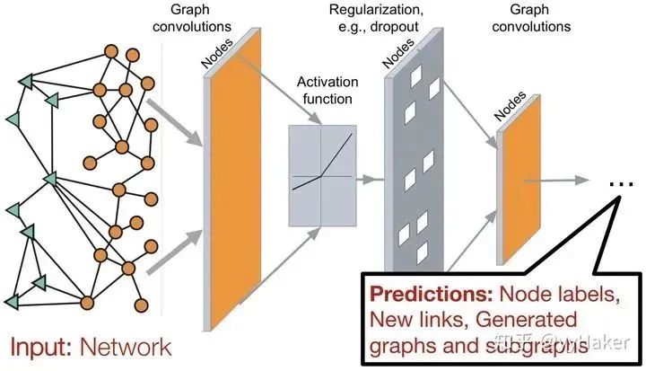
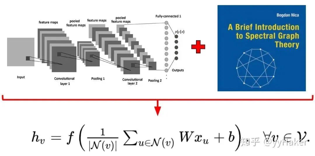
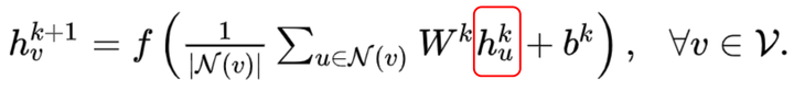
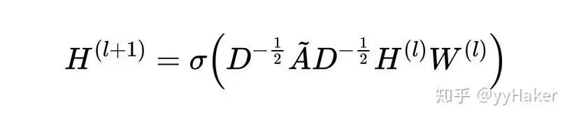
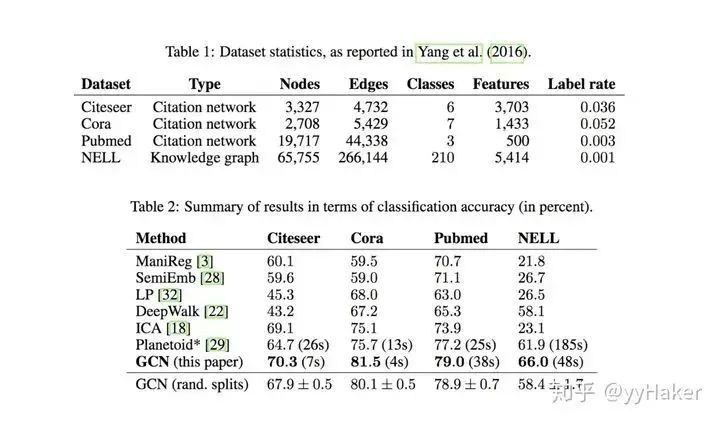 Figure 6
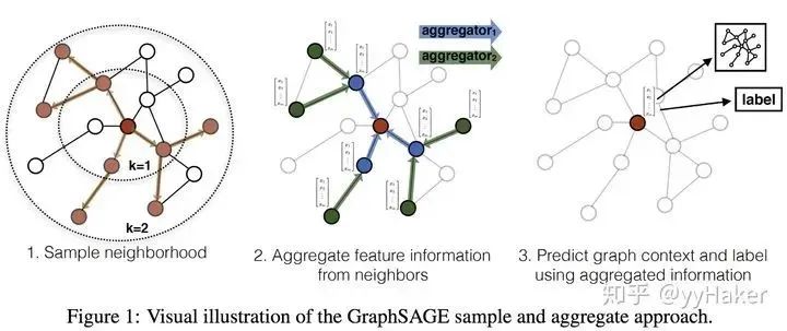
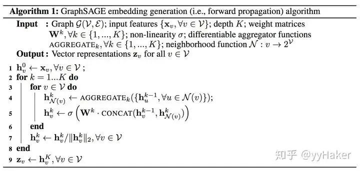
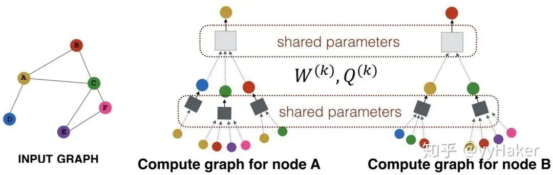
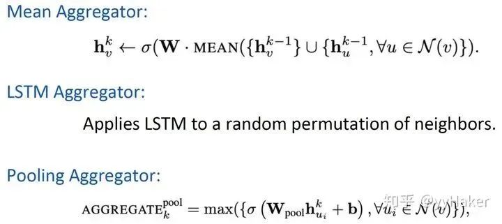
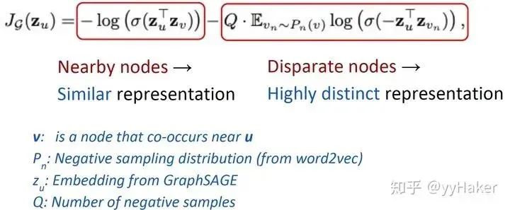
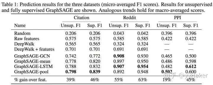
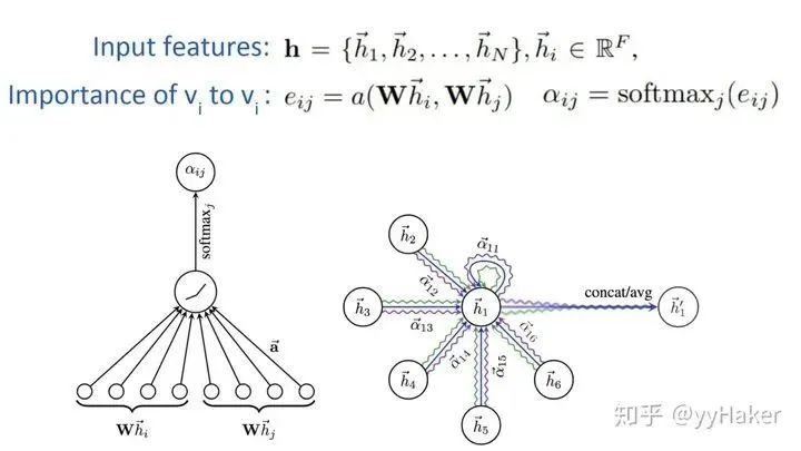 Figure 9