Understanding LSTM for Mathematical Competitions

In mathematical competitions, neural networks have gradually become a powerful assistant for participants due to their strong data processing and pattern recognition capabilities. Especially when dealing with complex, nonlinear, high-dimensional data, neural networks perform exceptionally well. They not only help us solve basic problems such as classification and regression, but also excel in advanced tasks like prediction and optimization. Among various neural network models, Long Short-Term Memory networks (LSTM) stand out for their unique structure and advantages in handling time series data.

Basic Concepts

LSTM, or Long Short-Term Memory network, is a special type of recurrent neural network (RNN). RNNs are a class of neural networks designed to handle sequential data, allowing information to be cyclically transmitted within the network, thereby capturing temporal dependencies in sequences. However, traditional RNNs often encounter issues of gradient vanishing or exploding when dealing with long sequential data, which leads to ineffective learning of long-term dependencies.

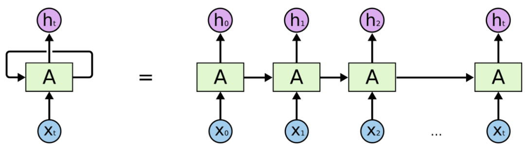
RNN Diagram

LSTM was created to solve this problem by introducing a unique gating mechanism, allowing the network to dynamically control the retention and forgetting of information, thus effectively learning long-term dependencies in sequences. Compared to traditional neural networks (such as Multi-Layer Perceptrons, MLP), LSTM has significant advantages in processing time series data. MLPs and other feedforward neural network structures are simple and suitable for static data or features that are independent of each other, while LSTM can handle data with clear temporal dependencies, such as stock prices, weather data, etc.

Core Explanation

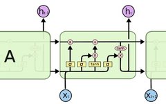
The key structure of LSTM lies in the “gates” mechanism within its units, which include the forget gate, input gate, and output gate. These gates control the flow of information through the Sigmoid function, allowing LSTM to dynamically decide which information should be retained and which should be forgotten.

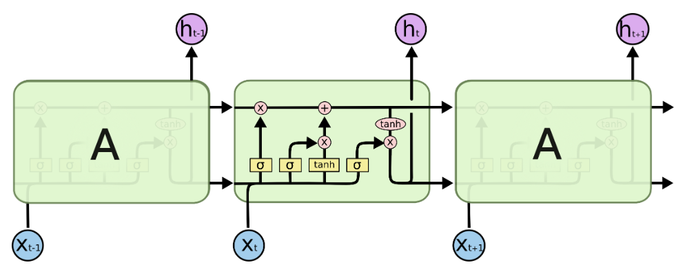
LSTM Diagram

1.Forget Gate: The forget gate determines which information from the previous cell state should be forgotten. Its calculation formula is:

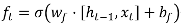
Where, ft is the output of the forget gate, σ is the Sigmoid function, Wf is the weight matrix of the forget gate, and [ht−1,xt] is the vector composed of the previous hidden state and the current input, while bf is the bias term.

2. Input Gate: The input gate determines which new information should be written into the cell state at the current moment. It first calculates the activation value of the input gate, then generates a new candidate cell state. The calculation formula is:

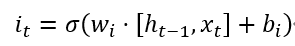
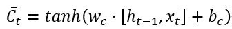
Where, the first equation is the output of the input gate, and the second equation is the new candidate cell state.

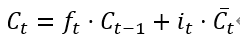
3. Updating the Cell State: Updating the cell state includes retaining part of the old cell state and adding the new cell state. The calculation formula is:

4. Output Gate: The output gate determines the current hidden state. It first calculates the activation value of the output gate, then computes the hidden state based on the cell state and activation value. The calculation formula is:

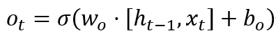
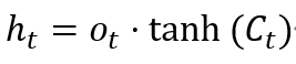
Where, ot is the output of the output gate, and ht is the current hidden state.

Through the above gating mechanism, LSTM can effectively solve the long-term dependency problem, allowing the network to remember input information from a long time ago and use that information in the current output.

Overview of Multi-Domain Applications

In addition to time series prediction tasks, LSTM is also widely used in Natural Language Processing (NLP), speech recognition, machine translation, and other fields. In the NLP field, LSTM can handle long-term dependencies in text data, achieving tasks such as text classification, sentiment analysis, text generation. In the speech recognition field, LSTM can convert speech signals into text information, enabling speech recognition functionality. In the machine translation field, LSTM can learn the correspondence between different languages, achieving automatic translation.

Real Case Study: 2024 E Problem

I. Problem Background

In the property insurance field, claim costs and the probability of extreme weather events are two important prediction targets. These predictions help insurance companies formulate more precise risk management and pricing strategies. The 2024 Mathematical Competition E problem involves predictions related to these two aspects.

II. Data Collection and Preprocessing

1. Data Collection:

Claim Data: Including historical claims records, claim amounts, reasons for claims, etc.

Weather Data: Including historical weather records, occurrence frequency and intensity of extreme weather events (such as hurricanes, heavy rains, droughts, etc.).

Geographic Location Information: Including latitude and longitude of the insured property, altitude, climate type, etc.

2. Data Preprocessing:

Data Cleaning: Remove outliers and missing values, and perform necessary interpolation or filling.

Feature Extraction: Extract features related to claim costs and extreme weather based on business needs, such as geographic location, house type, insurance rates, etc.

Data Normalization: Normalize feature data to the same scale to improve the convergence speed and prediction accuracy of the model.

III. LSTM Model Construction and Training

1. Model Construction:

Use Python’s Keras or TensorFlow framework to construct the LSTM model.

Set the number of LSTM layers, the number of neurons in each layer, activation functions, and other parameters.

Considering that claim costs and extreme weather are two different prediction targets, a multi-output LSTM model can be constructed to predict both targets simultaneously.

2. Model Training:

Divide the preprocessed data into training and testing sets.

Use the training set data to train the LSTM model, adjusting model parameters to minimize prediction errors.

Monitor the training process of the model, including changes in the loss function and performance on the validation set, to prevent overfitting.

IV. Model Evaluation and Prediction

1. Model Evaluation:

Use the testing set data to evaluate the prediction performance of the model.

Calculate the mean squared error (MSE), mean absolute error (MAE), and other metrics to measure the prediction accuracy of the model.

2. Prediction:

Use the trained LSTM model to predict claim costs and the probability of extreme weather events for the upcoming period.

Compare the prediction results with actual situations to verify the reliability and practicality of the model.

V. Result Analysis and Discussion

1. Result Analysis:

Analyze the accuracy of the prediction results, including the prediction accuracy of claim costs and the probability of extreme weather events.

Discuss the model’s performance across different time periods, regions, or house types to understand the model’s generalization ability.

2. Discussion:

Discuss the advantages and limitations of the LSTM model in property insurance forecasting.

Propose suggestions for improving model performance, such as increasing the number of features and optimizing model parameters.

Explore other potential applications of the LSTM model in the property insurance field, such as risk assessment and pricing strategy optimization.