Table of Contents
-
1. Neuron Model
-
2. Perceptron and Neural Networks
-
3. Error Backpropagation Algorithm
-
4. Common Neural Network Models
-
5. Deep Learning
-
6. References
Currently, deep learning (Deep Learning, referred to as DL) is exceptionally popular in the field of algorithms, not only in the internet and artificial intelligence but also in various fields of life, reflecting the significant transformation led by deep learning. To learn deep learning, one must first be familiar with some basic concepts of neural networks (Neural Networks, referred to as NN). Of course, the neural networks mentioned here are not biological neural networks; it seems more appropriate to refer to them as artificial neural networks (Artificial Neural Networks, referred to as ANN). Neural networks were initially an algorithm or model in the field of artificial intelligence, and have now developed into a multidisciplinary field that has regained attention and admiration with the progress made in deep learning.
Why do we say “regain”? In fact, neural networks have been researched as an algorithmic model for a long time, but after some progress, research on neural networks fell into a long period of decline. Later, with Hinton’s advancements in deep learning, neural networks regained people’s attention. This article focuses on neural networks, summarizing some related foundational knowledge, and then introducing the concept of deep learning. If there are any writing errors, please feel free to critique and correct.
1. Neuron Model
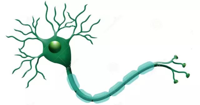
The neuron is the most basic structure in a neural network and can be said to be the basic unit of the neural network. Its design inspiration comes entirely from the information transmission mechanism of biological neurons. Students who have studied biology know that neurons have two states: excitation and inhibition. Generally, most neurons are in an inhibitory state, but once a neuron receives stimulation that causes its potential to exceed a threshold, that neuron will be activated and enter an “excited” state, subsequently spreading chemical substances (essentially information) to other neurons.
The diagram below illustrates the structure of a biological neuron:
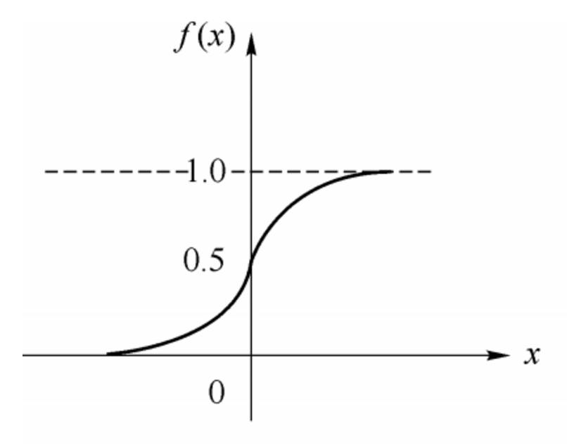
In 1943, McCulloch and Pitts represented the neuron structure in the above diagram with a simple model, forming an artificial neuron model, which is commonly referred to as the “M-P neuron model”, as shown in the diagram below:
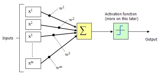
From the M-P neuron model shown above, we can see the output of the neuron
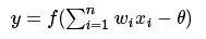
where is the activation threshold of the neuron mentioned earlier, and the function
The expression and distribution of the sigmoid function are shown below:
2. Perceptron and Neural Networks
The perceptron is a structure composed of two layers of neurons, where the input layer is used to accept external input signals, and the output layer (also referred to as the functional layer of the perceptron) is the M-P neuron. The diagram below represents a perceptron structure with an input layer consisting of three neurons (represented as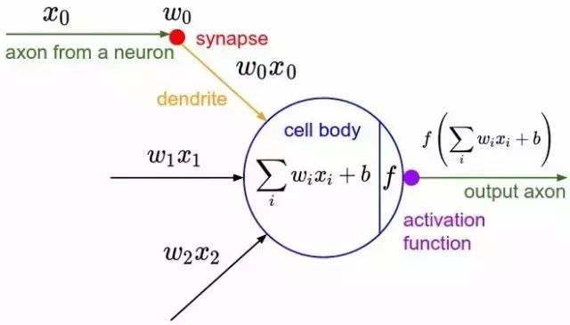
Based on the above diagram, it is easy to understand that the perceptron model can be represented by the following formula:
where
 However, since it only has one layer of functional neurons, its learning ability is very limited. It has been proven that a single-layer perceptron cannot solve even the simplest non-linearly separable problem—the XOR problem.
There is a historical context regarding the perceptron’s inability to solve the XOR problem that is worth briefly understanding: Perceptrons can only perform simple linear classification tasks. However, at that time, people’s enthusiasm was too high, and no one recognized this point clearly. Thus, when the artificial intelligence giant Minsky pointed this out, the situation changed. Minsky published a book titled “Perceptron” in 1969, in which he mathematically proved the weaknesses of perceptrons, especially their inability to solve simple classification tasks like XOR. Minsky believed that if the computational layers were increased to two layers, the computational load would be too great, and there would be no effective learning algorithms. Therefore, he thought that researching deeper networks was not valuable. Due to Minsky’s significant influence and the pessimistic attitude presented in the book, many scholars and laboratories abandoned research on neural networks. Research on neural networks fell into an ice age, known as the “AI winter.” Nearly ten years later, research on two-layer neural networks led to the revival of neural networks.
We know that many problems in our daily lives, even most of them, are not linearly separable. So how do we handle non-linearly separable problems? This is where we introduce the concept of “multi-layer.” Since a single-layer perceptron cannot solve non-linear problems, we use a multi-layer perceptron. The diagram below illustrates a two-layer perceptron solving the XOR problem:
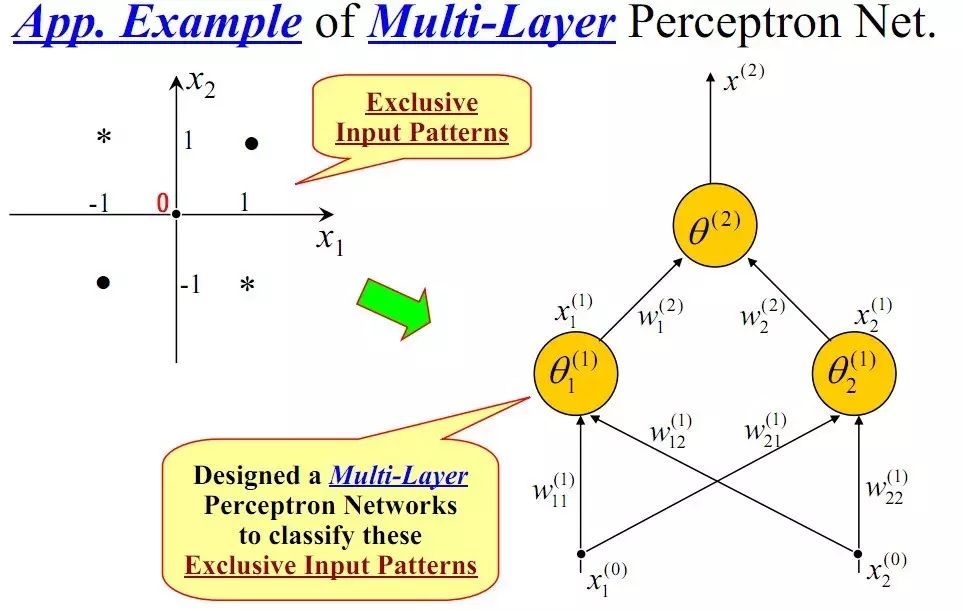
After constructing the above network, the final classification surface obtained through training is shown below:
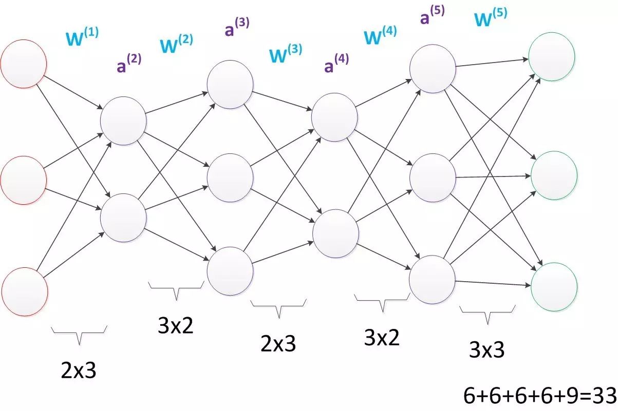
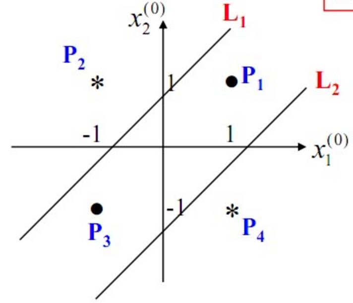 It can be seen that multi-layer perceptrons can effectively solve non-linearly separable problems. We typically refer to a multi-layer structure like a multi-layer perceptron as a neural network. However, as Minsky previously worried, although multi-layer perceptrons can theoretically solve non-linear problems, the complexity of real-life problems is far more than just the XOR problem. Therefore, we often need to construct multi-layer networks, and determining what learning algorithm to use for multi-layer neural networks is a significant challenge. As shown in the diagram below, a network with four hidden layers has at least 33 parameters (not counting the bias parameters). How should we determine these?
3. Error Backpropagation Algorithm
The so-called training or learning of neural networks mainly aims to obtain the parameters required by the neural network to solve specific problems through learning algorithms. These parameters include the connection weights between neurons in each layer and biases.
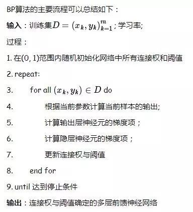
When talking about learning algorithms for neural networks, we must mention the most outstanding and successful representative—the error backpropagation (error BackPropagation, referred to as BP) algorithm. The BP learning algorithm is typically used in the most widely used multi-layer feedforward neural networks.
4. Common Neural Network Models
4.1 Boltzmann Machines and Restricted Boltzmann Machines
A class of models in neural networks defines an “energy” for the network state, where the network reaches an ideal state when the energy is minimized, and the training of the network involves minimizing this energy function. Boltzmann machines are energy-based models where the neurons are divided into two layers: visible and hidden. The visible layer represents the input and output of the data, while the hidden layer is understood as the intrinsic representation of the data. The neurons in Boltzmann machines are Boolean, meaning they can only take values of 0 or 1. Standard Boltzmann machines are fully connected, meaning that neurons within each layer are interconnected, leading to high computational complexity and difficulty in solving practical problems. Therefore, we often use a special type of Boltzmann machine—restricted Boltzmann machines (Restricted Boltzmann Machine, referred to as RBM), which have no connections within layers and connections between layers, and can be seen as a bipartite graph. The diagram below illustrates the structures of Boltzmann machines and RBMs:
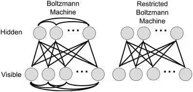
RBMs are often trained using contrastive divergence (Contrastive Divergence, referred to as CD).
4.2 RBF Networks
RBF (Radial Basis Function) networks are a type of single hidden layer feedforward neural network that uses radial basis functions as the activation functions for hidden layer neurons, while the output layer is a linear combination of the outputs of hidden layer neurons. The diagram below illustrates an RBF neural network:
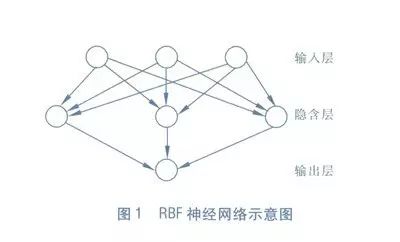 Training an RBF network typically involves two steps:
1> Determine the centers of the neurons, commonly using methods such as random sampling or clustering;
2> Determine the parameters of the neural network, commonly using the BP algorithm.
4.3 ART Networks
ART (Adaptive Resonance Theory) networks are important representatives of competitive learning. This network consists of a comparison layer, recognition layer, recognition layer threshold, and reset module. ART effectively alleviates the “stability-plasticity dilemma” in competitive learning, where plasticity refers to the ability of the neural network to learn new knowledge, while stability refers to the ability of the neural network to retain memory of old knowledge. This gives ART networks a significant advantage: they can perform incremental learning or online learning.
4.4 SOM Networks
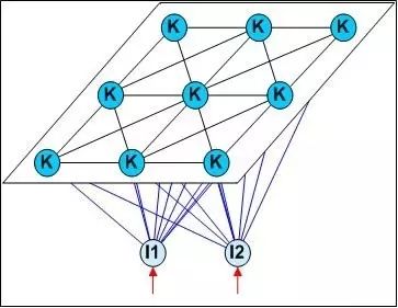
SOM (Self-Organizing Map) networks are a type of competitive learning-based unsupervised neural network that can map high-dimensional input data to a low-dimensional space (usually two-dimensional), while preserving the topological structure of the input data in high-dimensional space, meaning similar sample points in high-dimensional space are mapped to adjacent neurons in the network output layer. The diagram below illustrates the structure of SOM networks:
4.5 Structure Adaptive Networks
As mentioned earlier, typical neural networks specify the network structure in advance, and the training aims to determine suitable connection weights, thresholds, and other parameters using training samples. In contrast, structure adaptive networks treat the network structure as one of the learning objectives and hope to find a network structure that best fits the characteristics of the data during the training process.
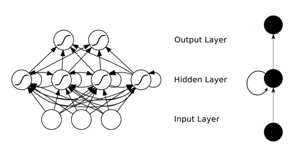
4.6 Recurrent Neural Networks and Elman Networks
Unlike feedforward neural networks, recurrent neural networks (Recurrent Neural Networks, referred to as RNN) allow for circular structures within the network, enabling some neurons’ outputs to feedback as input signals. This structure and information feedback process mean that the output state of the network at time
The Elman network is one of the most commonly used recurrent neural networks, structured as shown in the diagram below:
 The general training algorithm for RNNs uses an extended BP algorithm. It is worth mentioning that the result O(t+1) of the network at time (t+1) is the result of the input at that time and all historical interactions, achieving the purpose of modeling time series. Thus, in a certain sense, RNNs can be considered as deep learning in terms of temporal depth.
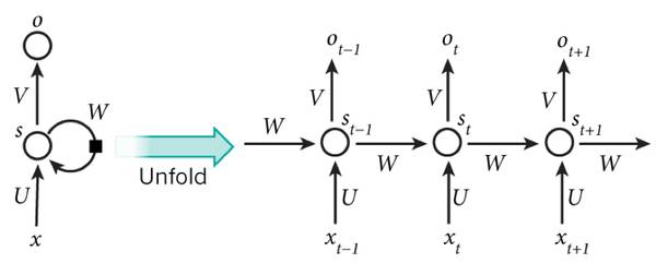 However, saying that the result O(t+1) of the network at time (t+1) is influenced by all history is not entirely accurate, as “gradient divergence” can also occur along the time axis. This means that for time t, the gradient produced may vanish after propagating through several layers in the time axis, failing to influence the distant past. Therefore, “all history” is only an ideal situation. In practice, this influence can only last for several time stamps. In other words, the error signal from later time steps often cannot return far enough into the past to influence the network, making it difficult to learn long-distance influences.
To address the gradient divergence along the time axis, the field of machine learning has developed long short-term memory units (Long-Short Term Memory, referred to as LSTM), which implement memory functions over time through gate switches and prevent gradient divergence. In fact, in addition to learning historical information, RNNs and LSTMs can also be designed into bidirectional structures, namely bidirectional RNNs and bidirectional LSTMs, utilizing both historical and future information.
5. Deep Learning
Deep learning refers to deep neural network models, typically indicating neural network structures with three or more layers.
Theoretically, the more parameters a model has, the higher its complexity and “capacity,” which means it can accomplish more complex learning tasks. Just like the insights from multi-layer perceptrons, the number of layers in a neural network directly determines its ability to represent reality. However, in general, complex models have low training efficiency and are prone to overfitting, making them less favored. Specifically, as the number of layers in a neural network increases, the optimization function is more likely to get trapped in local optima (i.e., overfitting, performing well on training samples but poorly on test sets). Additionally, an important issue is that as the number of layers increases, the phenomenon of “gradient vanishing” (or gradient divergence) becomes more severe. We often use the sigmoid function as the activation function for hidden layer neurons. For signals with an amplitude of 1, during BP backpropagation, the gradient diminishes to 0.25 with each layer. As the number of layers increases, gradients diminish exponentially, making it difficult for lower layers to receive effective training signals.
To solve the training issues of deep neural networks, an effective approach is to adopt unsupervised layer-wise training, where the basic idea is to train one hidden node layer at a time. During training, the output of the previous hidden node layer serves as the input, and the output of the current hidden node layer serves as the input for the next layer. This is known as “pre-training”; after pre-training is completed, the entire network undergoes “fine-tuning” training. For example, Hinton’s deep belief networks (Deep Belief Networks, referred to as DBN) consist of layers where each layer is an RBM, meaning the entire network can be viewed as a stack of several RBMs. During unsupervised training, the first layer is trained as an RBM model based on the training samples, which can be trained according to standard RBM methods; then, the pre-trained hidden nodes of the first layer are treated as input nodes for the second layer, and the second layer is pre-trained; … After pre-training is completed for all layers, the entire network is trained using the BP algorithm.
In fact, the “pre-training + fine-tuning” training method can be viewed as grouping a large number of parameters to first find locally optimal settings for each group, and then jointly optimizing based on these locally optimal results. This effectively utilizes the degrees of freedom provided by the model’s numerous parameters while saving training costs.
Another way to save training costs is through “weight sharing,” allowing a group of neurons to use the same connection weights. This strategy plays an important role in convolutional neural networks (Convolutional Neural Networks, referred to as CNN). The diagram below illustrates a CNN network:
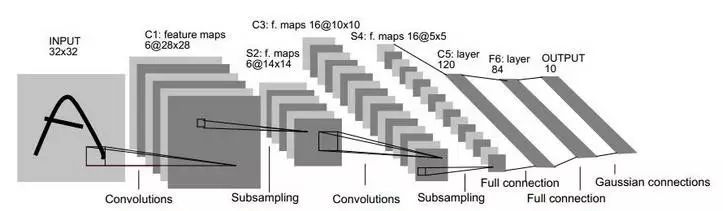 CNNs can be trained using the BP algorithm, but during training, whether in convolutional layers or sampling layers, each group of neurons (i.e., each “plane” in the diagram above) uses the same connection weights, significantly reducing the number of parameters that need to be trained.
6. References
1. Zhou Zhihua, “Machine Learning”
2. Zhihu Q&A: http://www.zhihu.com/question/34681168