Author: Shivam Bansal

Translated by: Shen Libin

Proofread by: Ding Nanya

This article is approximately 2300 words, and is recommended to be read in 8 minutes.

This article will detail the text classification problem and implement this process in Python.

Introduction

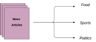
Text classification is a common natural language processing task in business problems, with the goal of automatically assigning text files to one or more predefined categories. Some examples of text classification include:

• Analyzing public sentiment in social media

• Identifying spam and non-spam emails

• Automatically labeling customer inquiries

• Categorizing news articles by topic

Table of Contents

This article will detail the text classification problem and implement this process in Python:

Text classification is an example of supervised learning, which uses a dataset containing text documents and labels to train a classifier. The end-to-end training of text classification mainly consists of three parts:

1. Preparing the dataset: The first step is to prepare the dataset, which includes loading the dataset and performing basic preprocessing, then splitting the dataset into a training set and a validation set.

Feature engineering: The second step is feature engineering, where the raw dataset is transformed into flat features for training machine learning models, and new features are created from existing data features.

2. Model training: The final step is modeling, where a machine learning model is trained using the labeled dataset.

3. Further improving classifier performance: This article will also discuss various methods to improve the performance of the text classifier.

Note: This article does not delve deeply into NLP tasks. If you want to review the basics first, you can refer to this article

https://www.analyticsvidhya.com/blog/2017/01/ultimate-guide-to-understand-implement-natural-language-processing-codes-in-python/

Prepare Your Machine

First, install the basic components to create a text classification framework in Python. Start by importing all the necessary libraries. If you haven’t installed these libraries, you can do so via the following official links.

• Pandas:https://pandas.pydata.org/pandas-docs/stable/install.html

• Scikit-learn:http://scikit-learn.org/stable/install.html

• XGBoost:http://xgboost.readthedocs.io/en/latest/build.html

• TextBlob:http://textblob.readthedocs.io/en/dev/install.html

• Keras:https://keras.io/#installation

# Import libraries needed for dataset preprocessing, feature engineering, and model training

from sklearn import model_selection, preprocessing, linear_model, naive_bayes, metrics, svm

from sklearn.feature_extraction.text import TfidfVectorizer, CountVectorizer

from sklearn import decomposition, ensemble

import pandas, xgboost, numpy, textblob, string

from keras.preprocessing import text, sequence

from keras import layers, models, optimizers

1. Preparing the Dataset

In this article, I use the Amazon review dataset, which can be downloaded from this link:

https://gist.github.com/kunalj101/ad1d9c58d338e20d09ff26bcc06c4235

This dataset contains 3.6M text reviews and their labels, and we will only use a small portion of it. First, load the downloaded data into a pandas data structure (dataframe) containing two columns (text and label).

Dataset link:

https://drive.google.com/drive/folders/0Bz8a_Dbh9Qhbfll6bVpmNUtUcFdjYmF2SEpmZUZUcVNiMUw1TWN6RDV3a0JHT3kxLVhVR2M

# Load the dataset

data = open(‘data/corpus’).read()

labels, texts = [], []

for i, line in enumerate(data.split(“\n”)):

content = line.split()

labels.append(content[0])

texts.append(content[1])

# Create a dataframe with columns named text and label

trainDF = pandas.DataFrame()

trainDF[‘text’] = texts

trainDF[‘label’] = labels

Next, we will split the dataset into training and validation sets so we can train and test the classifier. Additionally, we will encode our target column so that it can be used in machine learning models:

# Split the dataset into training and validation sets

train_x, valid_x, train_y, valid_y = model_selection.train_test_split(trainDF[‘text’], trainDF[‘label’])

# Label encoding for the target variable

encoder = preprocessing.LabelEncoder()

train_y = encoder.fit_transform(train_y)

valid_y = encoder.fit_transform(valid_y)

2. Feature Engineering

Next is feature engineering, where the raw data will be transformed into feature vectors, and new features will also be created based on existing data. To select important features from the dataset, there are several methods:

• Count vectors as features

• TF-IDF vectors as features

• Single word level

• Multiple word level (N-Gram)

• Part of speech level

• Word embeddings as features

• Text/NLP based features

• Topic models as features

Let’s take a look at how they are implemented:

2.1 Count Vectors as Features

Count vectors are a matrix representation of the dataset where each row represents a document from the corpus, each column represents a term from the corpus, and each cell represents the frequency count of a specific term in a specific document:

# Create a vector counter object

count_vect = CountVectorizer(analyzer=’word’, token_pattern=r’\w{1,}’)

count_vect.fit(trainDF[‘text’])

# Use the vector counter object to transform the training and validation sets

xtrain_count = count_vect.transform(train_x)

xvalid_count = count_vect.transform(valid_x)

2.2 TF-IDF Vectors as Features

The TF-IDF score represents the relative importance of a term in a document and across the entire corpus. The TF-IDF score consists of two parts: the first part calculates the standard term frequency (TF), and the second part is inverse document frequency (IDF). The IDF is calculated by dividing the total number of documents in the corpus by the number of documents containing the term, and then taking the logarithm.

TF(t) = (the number of times the term appears in the document) / (the total number of terms in the document)

IDF(t) = log_e (total number of documents / number of documents containing the term)

TF-IDF vectors can be generated from different levels of tokenization (single words, part of speech, multiple words (n-grams))

• Word Level TF-IDF: The matrix represents the TF-IDF score of each word across different documents.

• N-gram Level TF-IDF: N-grams are combinations of multiple words together, and this matrix represents the TF-IDF score of the N-grams.

• Part of Speech Level TF-IDF: The matrix represents the TF-IDF score of multiple parts of speech in the corpus.

# Word level TF-IDF

tfidf_vect = TfidfVectorizer(analyzer=’word’, token_pattern=r’\w{1,}’, max_features=5000)

tfidf_vect.fit(trainDF[‘text’])

xtrain_tfidf = tfidf_vect.transform(train_x)

xvalid_tfidf = tfidf_vect.transform(valid_x)

# N-gram level TF-IDF

tfidf_vect_ngram = TfidfVectorizer(analyzer=’word’, token_pattern=r’\w{1,}’, ngram_range=(2,3), max_features=5000)

tfidf_vect_ngram.fit(trainDF[‘text’])

xtrain_tfidf_ngram = tfidf_vect_ngram.transform(train_x)

xvalid_tfidf_ngram = tfidf_vect_ngram.transform(valid_x)

# Part of speech level TF-IDF

tfidf_vect_ngram_chars = TfidfVectorizer(analyzer=’char’, token_pattern=r’\w{1,}’, ngram_range=(2,3), max_features=5000)

tfidf_vect_ngram_chars.fit(trainDF[‘text’])

xtrain_tfidf_ngram_chars = tfidf_vect_ngram_chars.transform(train_x)

xvalid_tfidf_ngram_chars = tfidf_vect_ngram_chars.transform(valid_x)

2.3 Word Embeddings

Word embeddings are a form of representing words and documents using dense vectors. The position of words in the vector space is learned from the context in which the word appears in the text. Word embeddings can be trained using the input corpus itself or generated using pre-trained word embedding models such as Glove, FastText, and Word2Vec. They can all be downloaded and used with transfer learning. To learn more about word embeddings, you can visit:

https://www.analyticsvidhya.com/blog/2017/06/word-embeddings-count-word2veec/

Next, let’s see how to use a pre-trained word embedding model in the model, which mainly involves four steps:

1. Load the pre-trained word embedding model

2. Create a tokenizer object

3. Convert the text documents into sequences of tokens and pad them

4. Create a mapping of tokens to their respective embeddings

# Load the pre-trained word embedding vectors

embeddings_index = {}

for i, line in enumerate(open(‘data/wiki-news-300d-1M.vec’)):

values = line.split()

embeddings_index[values[0]] = numpy.asarray(values[1:], dtype=’float32′)

# Create a tokenizer

token = text.Tokenizer()

token.fit_on_texts(trainDF[‘text’])

word_index = token.word_index

# Convert the text to sequences of tokens and pad them to ensure uniform vector lengths

train_seq_x = sequence.pad_sequences(token.texts_to_sequences(train_x), maxlen=70)

valid_seq_x = sequence.pad_sequences(token.texts_to_sequences(valid_x), maxlen=70)

# Create the mapping of tokens to embeddings

embedding_matrix = numpy.zeros((len(word_index) + 1, 300))

for word, i in word_index.items():

embedding_vector = embeddings_index.get(word)

if embedding_vector is not None:

embedding_matrix[i] = embedding_vector

2.4 Text/NLP Based Features

Creating many additional text-based features can sometimes improve model performance. For example, the following:

• Word count of the document—Total number of words in the document

• Part of speech count of the document—Total number of parts of speech in the document

• Average word density of the document—Average length of words used in the document

• Total number of punctuation marks in the document—Total number of punctuation marks in the document

• Number of uppercase words in the entire document—Total number of uppercase words in the document

• Total number of titles in the entire document—Total number of appropriate topics (titles) in the document

• Frequency distribution of part of speech tagging

• Number of nouns

• Number of verbs

• Number of adjectives

• Number of adverbs

• Number of pronouns

These features are highly experimental and should be analyzed on a case-by-case basis.

trainDF[‘char_count’] = trainDF[‘text’].apply(len)

trainDF[‘word_count’] = trainDF[‘text’].apply(lambda x: len(x.split()))

trainDF[‘word_density’] = trainDF[‘char_count’] / (trainDF[‘word_count’]+1)

trainDF[‘punctuation_count’] = trainDF[‘text’].apply(lambda x: len(“”.join(_ for _ in x if _ in string.punctuation)))

trainDF[‘title_word_count’] = trainDF[‘text’].apply(lambda x: len([wrd for wrd in x.split() if wrd.istitle()]))

trainDF[‘upper_case_word_count’] = trainDF[‘text’].apply(lambda x: len([wrd for wrd in x.split() if wrd.isupper()]))

trainDF[‘char_count’] = trainDF[‘text’].apply(len)

trainDF[‘word_count’] = trainDF[‘text’].apply(lambda x: len(x.split()))

trainDF[‘word_density’] = trainDF[‘char_count’] / (trainDF[‘word_count’]+1)

trainDF[‘punctuation_count’] = trainDF[‘text’].apply(lambda x: len(“”.join(_ for _ in x if _ in string.punctuation)))

trainDF[‘title_word_count’] = trainDF[‘text’].apply(lambda x: len([wrd for wrd in x.split() if wrd.istitle()]))

trainDF[‘upper_case_word_count’] = trainDF[‘text’].apply(lambda x: len([wrd for wrd in x.split() if wrd.isupper()]))

pos_family = {

‘noun’: [‘NN’,’NNS’,’NNP’,’NNPS’],

‘pron’: [‘PRP’,’PRP$’,’WP’,’WP$’],

‘verb’: [‘VB’,’VBD’,’VBG’,’VBN’,’VBP’,’VBZ’],

‘adj’: [‘JJ’,’JJR’,’JJS’],

‘adv’: [‘RB’,’RBR’,’RBS’,’WRB’]

}

# Check and obtain the count of specific part of speech tags in a sentence

def check_pos_tag(x, flag):

cnt = 0

try:

wiki = textblob.TextBlob(x)

for tup in wiki.tags:

ppo = list(tup)[1]

if ppo in pos_family[flag]:

cnt += 1

except:

pass

return cnt

trainDF[‘noun_count’] = trainDF[‘text’].apply(lambda x: check_pos_tag(x, ‘noun’))

trainDF[‘verb_count’] = trainDF[‘text’].apply(lambda x: check_pos_tag(x, ‘verb’))

trainDF[‘adj_count’] = trainDF[‘text’].apply(lambda x: check_pos_tag(x, ‘adj’))

trainDF[‘adv_count’] = trainDF[‘text’].apply(lambda x: check_pos_tag(x, ‘adv’))

trainDF[‘pron_count’] = trainDF[‘text’].apply(lambda x: check_pos_tag(x, ‘pron’))

2.5 Topic Models as Features

Topic models are techniques for identifying phrases (topics) from a collection of documents that contain important information. I have used LDA to generate topic model features. LDA is an iterative model that starts with a fixed number of topics, each representing a distribution of terms, and each document representing a distribution of topics. Although the tokens themselves have no meaning, the probability distributions of the words expressed by the topics can convey the ideas of the document. For more information about topic models, please visit:

https://www.analyticsvidhya.com/blog/2016/08/beginners-guide-to-topic-modeling-in-python/

Let’s look at the process of running the topic model:

# Train the topic model

lda_model = decomposition.LatentDirichletAllocation(n_components=20, learning_method=’online’, max_iter=20)

X_topics = lda_model.fit_transform(xtrain_count)

topic_word = lda_model.components_

vocab = count_vect.get_feature_names()

# Visualize the topic model

n_top_words = 10

topic_summaries = []

for i, topic_dist in enumerate(topic_word):

topic_words = numpy.array(vocab)[numpy.argsort(topic_dist)][:-(n_top_words+1):-1]

topic_summaries.append(‘ ‘.join(topic_words)

3. Modeling

The final step of the text classification framework is to train a classifier using the features created earlier. There are many models available in machine learning for this final model. We will use the following different classifiers for text classification:

• Naive Bayes Classifier

• Linear Classifier

• Support Vector Machine (SVM)

• Bagging Models

• Boosting Models

• Shallow Neural Network

• Deep Neural Network

• Convolutional Neural Network (CNN)

• LSTM

• GRU

• Bidirectional RNN

• Recurrent Convolutional Neural Network (RCNN)

• Other variants of deep neural networks

Next, we will detail and use these models. The following function is a generic function for training models, where the input is the classifier, the feature vectors of the training data, the labels of the training data, and the feature vectors of the validation data. We use these inputs to train a model and calculate accuracy.

def train_model(classifier, feature_vector_train, label, feature_vector_valid, is_neural_net=False):

# Fit the training dataset on the classifier

classifier.fit(feature_vector_train, label)

# Predict the labels on the validation dataset

predictions = classifier.predict(feature_vector_valid)

if is_neural_net:

predictions = predictions.argmax(axis=-1)

return metrics.accuracy_score(predictions, valid_y)

3.1 Naive Bayes

Using the sklearn framework, we implement the Naive Bayes model under different features.

Naive Bayes is a classification technique based on Bayes’ theorem and assumes that the predictor variables are independent. The Naive Bayes classifier assumes that specific features within a category are independent of other existing features.

To learn more about the details of the Naive Bayes algorithm, click:

A Naive Bayes classifier assumes that the presence of a particular feature in a class is unrelated to the presence of any other feature

# Naive Bayes with count vector features

accuracy = train_model(naive_bayes.MultinomialNB(), xtrain_count, train_y, xvalid_count)

print “NB, Count Vectors: “, accuracy

# Naive Bayes with word-level TF-IDF vector features

accuracy = train_model(naive_bayes.MultinomialNB(), xtrain_tfidf, train_y, xvalid_tfidf)

print “NB, WordLevel TF-IDF: “, accuracy

# Naive Bayes with multiple word-level TF-IDF vector features

accuracy = train_model(naive_bayes.MultinomialNB(), xtrain_tfidf_ngram, train_y, xvalid_tfidf_ngram)

print “NB, N-Gram Vectors: “, accuracy

# Naive Bayes with part of speech level TF-IDF vector features

accuracy = train_model(naive_bayes.MultinomialNB(), xtrain_tfidf_ngram_chars, train_y, xvalid_tfidf_ngram_chars)

print “NB, CharLevel Vectors: “, accuracy

# Output results

NB, Count Vectors: 0.7004

NB, WordLevel TF-IDF: 0.7024

NB, N-Gram Vectors: 0.5344

NB, CharLevel Vectors: 0.6872

3.2 Linear Classifier

Implement a linear classifier (Logistic Regression): Logistic regression measures the relationship between the categorical dependent variable and one or more independent variables by estimating probabilities using the logistic/sigmoid function. To learn more about logistic regression, please visit:

https://www.analyticsvidhya.com/blog/2015/10/basics-logistic-regression/

# Linear Classifier on Count Vectors

accuracy = train_model(linear_model.LogisticRegression(), xtrain_count, train_y, xvalid_count)

print “LR, Count Vectors: “, accuracy

# Linear classifier with word-level TF-IDF vector features

accuracy = train_model(linear_model.LogisticRegression(), xtrain_tfidf, train_y, xvalid_tfidf)

print “LR, WordLevel TF-IDF: “, accuracy

# Linear classifier with multiple word-level TF-IDF vector features

accuracy = train_model(linear_model.LogisticRegression(), xtrain_tfidf_ngram, train_y, xvalid_tfidf_ngram)

print “LR, N-Gram Vectors: “, accuracy

# Linear classifier with part of speech level TF-IDF vector features

accuracy = train_model(linear_model.LogisticRegression(), xtrain_tfidf_ngram_chars, train_y, xvalid_tfidf_ngram_chars)

print “LR, CharLevel Vectors: “, accuracy

# Output results

LR, Count Vectors: 0.7048

LR, WordLevel TF-IDF: 0.7056

LR, N-Gram Vectors: 0.4896

LR, CharLevel Vectors: 0.7012

3.3 Implementing Support Vector Machine Model

Support Vector Machines (SVM) are a type of supervised learning algorithm that can be used for classification or regression. This model extracts the best hyperplane or line that separates the two classes. To learn more about SVM, please visit:

https://www.analyticsvidhya.com/blog/2017/09/understaing-support-vector-machine-example-code/

# SVM with multiple word-level TF-IDF vector features

accuracy = train_model(svm.SVC(), xtrain_tfidf_ngram, train_y, xvalid_tfidf_ngram)

print “SVM, N-Gram Vectors: “, accuracy

# Output results

SVM, N-Gram Vectors: 0.5296

3.4 Bagging Model

Implement a Random Forest model: Random Forest is an ensemble model, more accurately a Bagging model. It is part of the family of tree models. To learn more about Random Forest, please visit:

https://www.analyticsvidhya.com/blog/2014/06/introduction-random-forest-simplified/

# Random Forest with count vector features

accuracy = train_model(ensemble.RandomForestClassifier(), xtrain_count, train_y, xvalid_count)

print “RF, Count Vectors: “, accuracy

# Random Forest with word-level TF-IDF vector features

accuracy = train_model(ensemble.RandomForestClassifier(), xtrain_tfidf, train_y, xvalid_tfidf)

print “RF, WordLevel TF-IDF: “, accuracy

# Output results

RF, Count Vectors: 0.6972

RF, WordLevel TF-IDF: 0.6988

3.5 Boosting Model

Implement an Xgboost model: Boosting models are another type of tree-based ensemble model. Boosting is a machine learning ensemble meta-algorithm primarily used to reduce bias in models. It is a set of machine learning algorithms that can elevate weak learners to strong learners, where weak learners refer to classifiers that are only slightly better than random guessing. To learn more, please visit:

https://www.analyticsvidhya.com/blog/2016/01/xgboost-algorithm-easy-steps/

# Xgboost with count vector features

accuracy = train_model(xgboost.XGBClassifier(), xtrain_count.tocsc(), train_y, xvalid_count.tocsc())

print “Xgb, Count Vectors: “, accuracy

# Xgboost with word-level TF-IDF vector features

accuracy = train_model(xgboost.XGBClassifier(), xtrain_tfidf.tocsc(), train_y, xvalid_tfidf.tocsc())

print “Xgb, WordLevel TF-IDF: “, accuracy

# Xgboost with part of speech level TF-IDF vector features

accuracy = train_model(xgboost.XGBClassifier(), xtrain_tfidf_ngram_chars.tocsc(), train_y, xvalid_tfidf_ngram_chars.tocsc())

print “Xgb, CharLevel Vectors: “, accuracy

# Output results

Xgb, Count Vectors: 0.6324

Xgb, WordLevel TF-IDF: 0.6364

Xgb, CharLevel Vectors: 0.6548

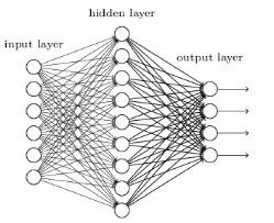
3.6 Shallow Neural Network

Neural networks are designed as mathematical models that resemble biological neurons and the nervous system, used to discover complex patterns and relationships present in labeled data. A shallow neural network mainly consists of three layers of neurons—input layer, hidden layer, and output layer. To learn more about shallow neural networks, please visit:

https://www.analyticsvidhya.com/blog/2017/05/neural-network-from-scratch-in-python-and-r/

def create_model_architecture(input_size):

# create input layer

input_layer = layers.Input((input_size, ), sparse=True)

# create hidden layer

hidden_layer = layers.Dense(100, activation=”relu”)(input_layer)

# create output layer

output_layer = layers.Dense(1, activation=”sigmoid”)(hidden_layer)

classifier = models.Model(inputs = input_layer, outputs = output_layer)

classifier.compile(optimizer=optimizers.Adam(), loss=’binary_crossentropy’)

return classifier

classifier = create_model_architecture(xtrain_tfidf_ngram.shape[1])

accuracy = train_model(classifier, xtrain_tfidf_ngram, train_y, xvalid_tfidf_ngram, is_neural_net=True)

print “NN, Ngram Level TF IDF Vectors”, accuracy

# Output results:

Epoch 1/1

7500/7500 [==============================] – 1s 67us/step – loss: 0.6909

NN, Ngram Level TF IDF Vectors 0.5296

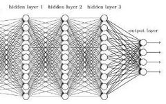
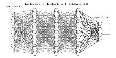
3.7 Deep Neural Network

Deep neural networks are more complex neural networks where the hidden layers perform more complex operations than simple sigmoid or ReLU activation functions. Different types of deep learning models can be applied to text classification problems.

• Convolutional Neural Network

In Convolutional Neural Networks, convolutions on the input layer are used to compute the output. In the local connection results, each input unit connects to the output neurons. Each layer of the network applies different filters and combines their results.

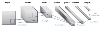
To learn more about Convolutional Neural Networks, please visit:

https://www.analyticsvidhya.com/blog/2017/06/architecture-of-convolutional-neural-networks-simplified-demystified/

def create_cnn():

# Add an Input Layer

input_layer = layers.Input((70, ))

# Add the word embedding Layer

embedding_layer = layers.Embedding(len(word_index) + 1, 300, weights=[embedding_matrix], trainable=False)(input_layer)

embedding_layer = layers.SpatialDropout1D(0.3)(embedding_layer)

# Add the convolutional Layer

conv_layer = layers.Convolution1D(100, 3, activation=”relu”)(embedding_layer)

# Add the pooling Layer

pooling_layer = layers.GlobalMaxPool1D()(conv_layer)

# Add the output Layers

output_layer1 = layers.Dense(50, activation=”relu”)(pooling_layer)

output_layer1 = layers.Dropout(0.25)(output_layer1)

output_layer2 = layers.Dense(1, activation=”sigmoid”)(output_layer1)

# Compile the model

model = models.Model(inputs=input_layer, outputs=output_layer2)

model.compile(optimizer=optimizers.Adam(), loss=’binary_crossentropy’)

return model

classifier = create_cnn()

accuracy = train_model(classifier, train_seq_x, train_y, valid_seq_x, is_neural_net=True)

print “CNN, Word Embeddings”, accuracy

# Output results

Epoch 1/1

7500/7500 [==============================] – 12s 2ms/step – loss: 0.5847

CNN, Word Embeddings 0.5296

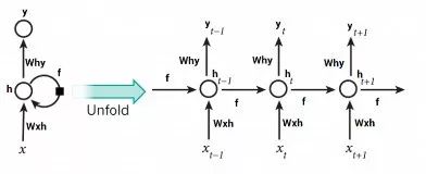
• Recurrent Neural Network – LSTM

Unlike feedforward neural networks, where the activation output propagates in one direction, recurrent neural networks propagate the activation output in both directions (from input to output and from output to input). This creates a cycle in the neural network architecture, acting as a “memory state” of the neurons, allowing them to remember what they have learned so far. The memory state in RNNs is superior to traditional neural networks; however, a problem called gradient vanishing also arises due to this architecture. This problem makes it difficult to learn and adjust the parameters of earlier network layers when the network has many layers. To solve this problem, a new type of RNN model called LSTM (Long Short Term Memory) was developed:

To learn more about LSTM, please visit:

https://www.analyticsvidhya.com/blog/2017/12/fundamentals-of-deep-learning-introduction-to-lstm/

def create_rnn_lstm():

# Add an Input Layer

input_layer = layers.Input((70, ))

# Add the word embedding Layer

embedding_layer = layers.Embedding(len(word_index) + 1, 300, weights=[embedding_matrix], trainable=False)(input_layer)

embedding_layer = layers.SpatialDropout1D(0.3)(embedding_layer)

# Add the LSTM Layer

lstm_layer = layers.LSTM(100)(embedding_layer)

# Add the output Layers

output_layer1 = layers.Dense(50, activation=”relu”)(lstm_layer)

output_layer1 = layers.Dropout(0.25)(output_layer1)

output_layer2 = layers.Dense(1, activation=”sigmoid”)(output_layer1)

# Compile the model

model = models.Model(inputs=input_layer, outputs=output_layer2)

model.compile(optimizer=optimizers.Adam(), loss=’binary_crossentropy’)

return model

classifier = create_rnn_lstm()

accuracy = train_model(classifier, train_seq_x, train_y, valid_seq_x, is_neural_net=True)

print “RNN-LSTM, Word Embeddings”, accuracy

# Output results

Epoch 1/1

7500/7500 [==============================] – 22s 3ms/step – loss: 0.6899

RNN-LSTM, Word Embeddings 0.5124

• Recurrent Neural Network – GRU

Gated Recurrent Units are another form of recurrent neural networks, and we add a GRU layer to the network instead of LSTM.

def create_rnn_gru():

# Add an Input Layer

input_layer = layers.Input((70, ))

# Add the word embedding Layer

embedding_layer = layers.Embedding(len(word_index) + 1, 300, weights=[embedding_matrix], trainable=False)(input_layer)

embedding_layer = layers.SpatialDropout1D(0.3)(embedding_layer)

# Add the GRU Layer

lstm_layer = layers.GRU(100)(embedding_layer)

# Add the output Layers

output_layer1 = layers.Dense(50, activation=”relu”)(lstm_layer)

output_layer1 = layers.Dropout(0.25)(output_layer1)

output_layer2 = layers.Dense(1, activation=”sigmoid”)(output_layer1)

# Compile the model

model = models.Model(inputs=input_layer, outputs=output_layer2)

model.compile(optimizer=optimizers.Adam(), loss=’binary_crossentropy’)

return model

classifier = create_rnn_gru()

accuracy = train_model(classifier, train_seq_x, train_y, valid_seq_x, is_neural_net=True)

print “RNN-GRU, Word Embeddings”, accuracy

# Output results

Epoch 1/1

7500/7500 [==============================] – 19s 3ms/step – loss: 0.6898

RNN-GRU, Word Embeddings 0.5124

• Bidirectional RNN

The RNN layer can also be wrapped in a bidirectional layer; we wrap the GRU layer in a bidirectional RNN network.

def create_bidirectional_rnn():

# Add an Input Layer

input_layer = layers.Input((70, ))

# Add the word embedding Layer

embedding_layer = layers.Embedding(len(word_index) + 1, 300, weights=[embedding_matrix], trainable=False)(input_layer)

embedding_layer = layers.SpatialDropout1D(0.3)(embedding_layer)

# Add the LSTM Layer

lstm_layer = layers.Bidirectional(layers.GRU(100))(embedding_layer)

# Add the output Layers

output_layer1 = layers.Dense(50, activation=”relu”)(lstm_layer)

output_layer1 = layers.Dropout(0.25)(output_layer1)

output_layer2 = layers.Dense(1, activation=”sigmoid”)(output_layer1)

# Compile the model

model = models.Model(inputs=input_layer, outputs=output_layer2)

model.compile(optimizer=optimizers.Adam(), loss=’binary_crossentropy’)

return model

classifier = create_bidirectional_rnn()

accuracy = train_model(classifier, train_seq_x, train_y, valid_seq_x, is_neural_net=True)

print “RNN-Bidirectional, Word Embeddings”, accuracy

# Output results

Epoch 1/1

7500/7500 [==============================] – 32s 4ms/step – loss: 0.6889

RNN-Bidirectional, Word Embeddings 0.5124

• Recurrent Convolutional Neural Network

If the basic architecture has already been attempted, you can try different variants of these layers, such as recurrent convolutional neural networks and other variants, such as:

• Sequence to Sequence Models with Attention

• Sequence to Sequence Models with Attention using Attention Mechanism

• Bidirectional Recurrent Convolutional Neural Networks

• More layers of CNNs and RNNs

def create_rcnn():

# Add an Input Layer

input_layer = layers.Input((70, ))

# Add the word embedding Layer

embedding_layer = layers.Embedding(len(word_index) + 1, 300, weights=[embedding_matrix], trainable=False)(input_layer)

embedding_layer = layers.SpatialDropout1D(0.3)(embedding_layer)

# Add the recurrent layer

rnn_layer = layers.Bidirectional(layers.GRU(50, return_sequences=True))(embedding_layer)

# Add the convolutional Layer

conv_layer = layers.Convolution1D(100, 3, activation=”relu”)(embedding_layer)

# Add the pooling Layer

pooling_layer = layers.GlobalMaxPool1D()(conv_layer)

# Add the output Layers

output_layer1 = layers.Dense(50, activation=”relu”)(pooling_layer)

output_layer1 = layers.Dropout(0.25)(output_layer1)

output_layer2 = layers.Dense(1, activation=”sigmoid”)(output_layer1)

# Compile the model

model = models.Model(inputs=input_layer, outputs=output_layer2)

model.compile(optimizer=optimizers.Adam(), loss=’binary_crossentropy’)

return model

classifier = create_rcnn()

accuracy = train_model(classifier, train_seq_x, train_y, valid_seq_x, is_neural_net=True)

print “CNN, Word Embeddings”, accuracy

# Output results

Epoch 1/1

7500/7500 [==============================] – 11s 1ms/step – loss: 0.6902

CNN, Word Embeddings 0.5124

Further Improving the Performance of Text Classification Models

Although the above framework can be applied to multiple text classification problems, to achieve higher accuracy, some improvements can be made to the overall framework. For example, here are some tips to improve the performance of text classification models and the framework:

1. Clean the Text: Text cleaning helps reduce noise present in the text data, including stop words, punctuation, suffix variations, etc. This article helps to understand how to implement text classification:

https://www.analyticsvidhya.com/blog/2014/11/text-data-cleaning-steps-python/

2. Combine Text Feature Vectors with Text/NLP Features: During the feature engineering phase, combining the generated text feature vectors may improve the accuracy of the text classifier.

Tuning hyperparameters in the model: Hyperparameter tuning is an important step; many parameters can achieve the best fitting model through suitable tuning, such as tree depth, number of leaf nodes, network parameters, etc.

3. Ensemble Models: Stacking different models and mixing their outputs helps further improve results. To learn more about model ensembles, please visit:

https://www.analyticsvidhya.com/blog/2015/08/introduction-ensemble-learning/

Conclusion

This article discussed how to prepare a text dataset, including cleaning, creating training and validation sets. It utilized various types of feature engineering, such as count vectors, TF-IDF, word embeddings, topic models, and basic text features. Then, multiple classifiers were trained, including Naive Bayes, Logistic Regression, SVM, MLP, LSTM, and GRU. Finally, various methods to improve the performance of the text classifier were discussed.

Did you benefit from this article? Feel free to share your thoughts and opinions in the comments below.

Original link: https://www.analyticsvidhya.com/blog/2018/04/a-comprehensive-guide-to-understand-and-implement-text-classification-in-python/

Translator’s Bio

Shen Libin, a graduate student, primarily researching big data machine learning. Currently learning about the application of deep learning in NLP, hoping to learn and progress with friends who are interested in big data on the THU Datapi platform.

Translation Group Recruitment Information

Job Content: Requires a meticulous heart to translate selected foreign articles into fluent Chinese. If you are a data science/statistics/computer science student abroad, or working overseas in related fields, or confident in your foreign language skills, you are welcome to join the translation team.

You will gain: Regular translation training to improve volunteers’ translation skills, enhance awareness of cutting-edge data science, and overseas friends can stay connected with domestic technical application development. The THU Datapi’s industry-academia-research background offers good development opportunities for volunteers.

Other Benefits: Data scientists from well-known companies, students from Peking University, Tsinghua University, and other prestigious institutions will become your partners in the translation team.

Click the “Read Original” at the end of the article to join the Datapi team~

Reprint Notice

If you need to reprint, please indicate the author and source (reprinted from: Datapi ID: datapi) in a prominent position at the beginning of the article, and place a prominent QR code for Datapi at the end of the article. For articles with original identification, please send [Article Name – Pending Authorized Public Account Name and ID] to the contact email to apply for whitelist authorization and edit as required.

After publishing, please provide the link feedback to the contact email (see below). Unauthorized reprints and adaptations will be legally pursued.

Click “Read Original” to embrace the organization