
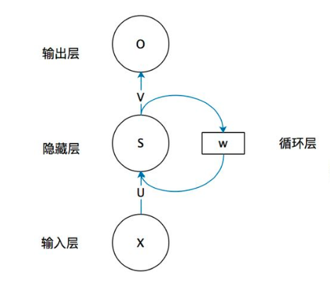
Recurrent Neural Networks (RNN) are designed based on the recursive nature of sequential data (such as language, speech, and time series) and are a type of feedback neural network that contains loops and self-repetitions, hence the name “recurrent”. They are specifically used to handle sequential data, such as generating text word by word or predicting time series data (e.g., stock prices).
1. Types of RNN Networks
RNN can be classified into five basic structural types based on the different number of inputs (m) corresponding to outputs (n):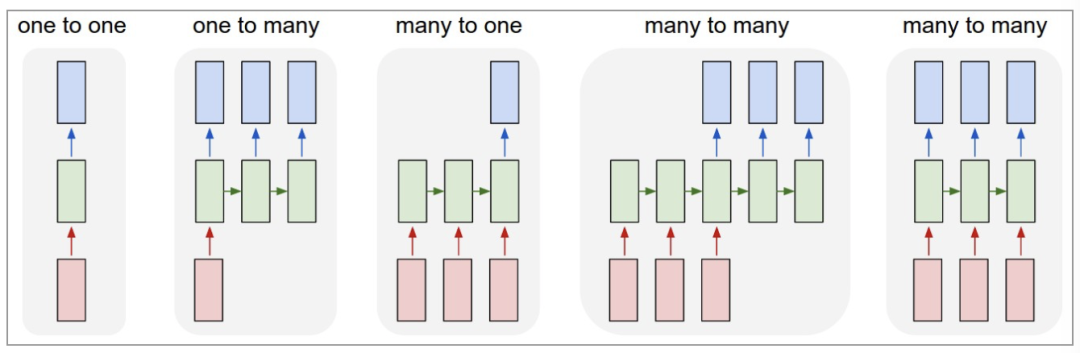
(1) One to One: This is essentially no different from a fully connected neural network and does not count as RNN.
(2) One to Many: The input is not a sequence, but the output is a sequence. This can be used for generating articles or music by theme.
(3) Many to One: The input is a sequence, but the output is not a sequence (it is a single value). Commonly used for text classification and regression prediction.
(4) Many to Many: Both the input and output are sequences of variable lengths. This is the Encoder-Decoder structure, commonly used in machine translation.
(5) Many to Many (m==n): Both the input and output are sequences of the same length. This is the most classic structural type in RNN, often used for named entity recognition and sequence prediction in NLP.
2. Principles of RNN
Regarding the RNN model, we will analyze it from the aspects of data, model, learning objectives, and optimization algorithms, focusing on the differences between its inputs and outputs (this section uses the classic m==n RNN structure as an example).
2.1 Data Level
Unlike traditional machine learning models that assume inputs are independent, RNN’s input data elements have order and interdependence, and are inputted into the model serially at each time step. The input from the previous step affects the prediction for the next step (for example, in a text prediction task, for the sequence “The cat eats fish”, the previous input “The cat”–x(0) will affect the probability of predicting the next word “eats”–x(1), and will continue to influence the prediction of the subsequent word “fish”–x(2)). Through the RNN structure, we can feedback historical (contextual) information to the next step.
2.2 Model Level and Forward Propagation
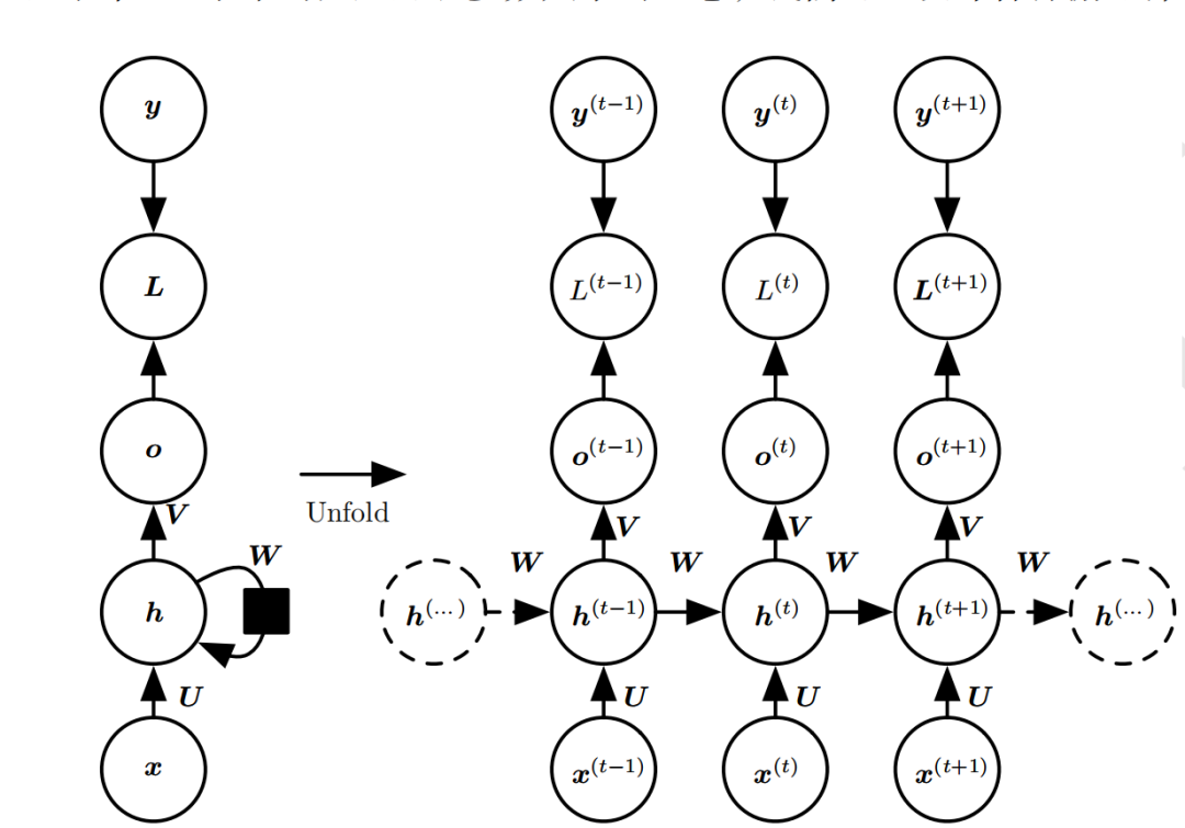
As shown in the figure, the RNN model (such as the left model, in fact, there is only one physical model), can be unfolded at each time step (as shown in the right model), and can be seen as multiple fully connected neural networks linked and sharing () parameters over time steps. The unfolded 3D diagram is as follows: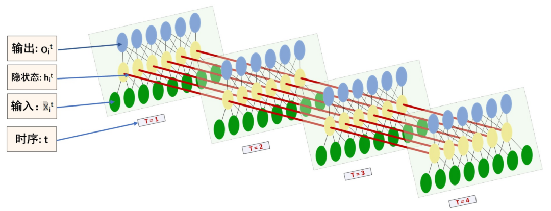
In addition to accepting the input x(t) at each step, RNN also connects the feedback information from the previous input—the hidden state h(t-1). The current hidden state ℎ(t) at the current moment is determined by the current input x(t) and the previous hidden state h(t-1).
Additionally, the RNN neurons share the weight parameter matrix at each time step (unlike CNN which shares parameters in space). The time dimension’s parameter sharing can fully utilize the temporal correlations between the data. If we had a separate parameter for each time point, it would not generalize to unseen sequence lengths during training, nor would it share statistical strengths across different sequence lengths and positions over time.
The following forward propagation computation flow chart for each time step will be broken down step by step: 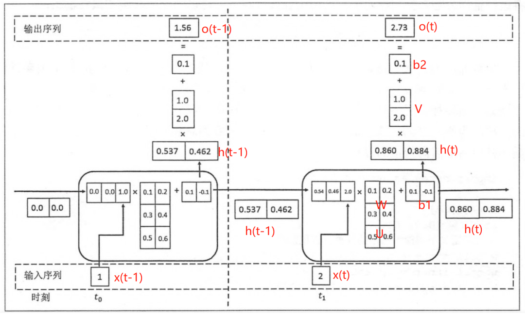
The above diagram expands the computation processes for two time steps t-1 and t;
t takes values from 0 to m (the length of the sequence);
x(t) is the input vector at time step t;
U is the weight matrix from the input layer to the hidden layer;
h(t) is the output state vector of the hidden layer at time step t, representing the feedback information of historical inputs (context);
V is the weight matrix from the hidden layer to the output layer; b is the bias term;
o(t) is the output vector of the output layer at time step t;
2.2.1 Input Process at Time Step t
Assuming the state h at each time step has a dimension of 2, the initial value of h is [0,0], and the input x and output o have a dimension of 1.
The state from the previous moment h(t-1) is concatenated with the current input x(t) to form a one-dimensional vector as the input to the fully connected hidden layer, corresponding to the input dimension of the hidden layer being 3 (as shown in the input part of the figure below).
2.2.2 Output h(t) at Time Step t and Feedback to the Next Step
Corresponding to the computation flow chart, the output state h(t-1) at time t-1 is [0.537, 0.462], and the input at time t is [2.0]. After concatenation, it becomes [0.537, 0.462, 2.0] as input to the fully connected hidden layer. The weight matrix for the hidden layer is [[0.1, 0.2], [0.3, 0.4], [0.5, 0.6]], and the bias term b1 is [0.1, -0.1]. The matrix operation through the hidden layer is: h(t-1) concatenated with x(t) * weight parameter W concatenated with weight matrix U + bias term (b1), then output state h(t) after tanh transformation. Next, h(t) and x(t+1) continue to be input to the hidden layer for the next step (t+1).
# Matrix operation code for the hidden layer
np.tanh(np.dot(np.array([[0.537, 0.462, 2.0]]),np.array([[0.1, 0.2], [0.3, 0.4], [0.5, 0.6]])) + np.array([0.1, -0.1]))
# Output h(t) is: array([[0.85972772, 0.88365397]])
2.2.3 Process from h(t) at Time Step t to Output o(t)
The hidden layer output state h(t) is [0.86, 0.884], and the output layer weight matrix is [[1.0], [2.0]], with the bias term b1 being [0.1]. The output layer’s matrix operation is: h(t) * V + bias term (b2) then outputs o(t).
# Matrix operation code for the output layer
np.dot(np.array([[0.85972772, 0.88365397]]),np.array([[1.0], [2.0]])) + np.array([0.1])
# o(t) output: array([[2.72703566]])
The above process traverses from the initial input (t=0) to the end of the sequence (t=m), which constitutes a complete forward propagation process. We can see that the weight matrices and bias terms are the same group at different moments, indicating that RNN shares parameters at different moments.
This RNN computation process can be briefly summarized with two formulas:
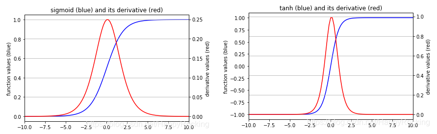
State h(t) = f(U * x(t) + W * h(t-1) + b1), where f is the activation function, and the hidden layer uses tanh in the above diagram. Common activation functions for hidden layers include tanh and relu.
Output o(t) = g(V * h(t) + b2), where g is the activation function. The output layer performs regression prediction without using a nonlinear activation function. When used for classification tasks, the output layer generally uses the softmax activation function.
2.3 Learning Objectives
After mapping the input x(t) sequence to the output value o(t), similar to fully connected neural networks, we can measure the error between each o(t) and the corresponding training target y (e.g., cross-entropy, mean squared error) as the loss function, aiming to minimize the loss function L(U,W,V) as the learning objective (also referred to as the optimization strategy).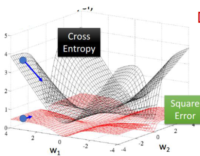
2.4 Optimization Algorithm
The optimization process of RNN is not fundamentally different from that of fully connected neural networks. It involves backpropagation of errors and multiple iterations of gradient descent to optimize parameters to obtain suitable RNN model parameters (bias terms are ignored here).
The difference is that RNN is based on time backpropagation, so the backpropagation of RNN is sometimes also called BPTT (back-propagation through time). BPTT sums the gradients at different time steps, and since all parameters are shared at various positions in the sequence, we update the same group of parameters during backpropagation. The following is a diagram illustrating BPTT and the process of deriving (gradients) for U, W, and V.
Optimizing parameters is relatively simple, deriving the partial derivative of parameters, and summing gradients at different time steps: The derivation of the partial derivative for is relatively complex as it involves historical data. Assuming there are only three moments (t==3), the partial derivative of at the third moment is:

Correspondingly, the partial derivative of U at the third moment is:
Based on the above two formulas, we can write the general formula for L’s partial derivatives with respect to at time and :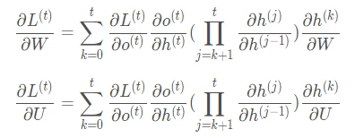
-
Difficulties in RNN Optimization
2.5 Limitations of RNN
-
The above shows a unidirectional RNN, which has a drawback that at time t, it cannot use the sequence information from time t+1 and beyond, leading to the development of bidirectional recurrent neural networks (bidirectional RNN).
-
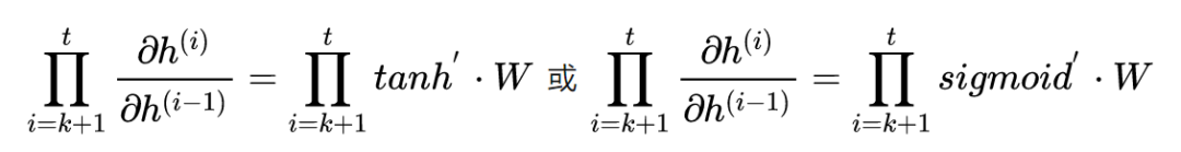
Theoretically, RNN can utilize information from sequences of any length, but in practice, the length it can remember is limited. After a certain period, it leads to gradient explosion or vanishing (as discussed in the previous section), which is known as the long-term dependencies problem. Generally, using traditional RNN requires limiting the maximum length of sequences, setting gradient clipping, and regularizing the flow of information, or using gated RNNs like GRU and LSTM to address the long-term dependencies problem (to be discussed in later topics).
3. RNN Stock Prediction
This project creates a single-layer hidden RNN model that inputs the time series data of stock opening prices for the previous 60 trading days (time steps) to predict the opening price for the next (60+1) trading day.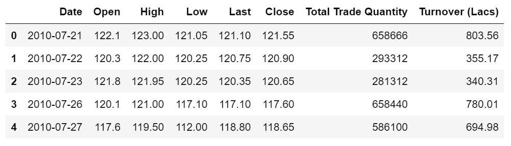
Import stock data and select the time series data of stock opening prices.
import numpy as np
import matplotlib.pyplot as plt
import pandas as pd

# (Read the original article of this public account to access the dataset and source code)
dataset_train = pd.read_csv('./data/NSE-TATAGLOBAL.csv')
dataset_train = dataset_train.sort_values(by='Date').reset_index(drop=True)
training_set = dataset_train.iloc[:, 1:2].values
print(dataset_train.shape)
dataset_train.head()
Normalize the training data to accelerate network training convergence.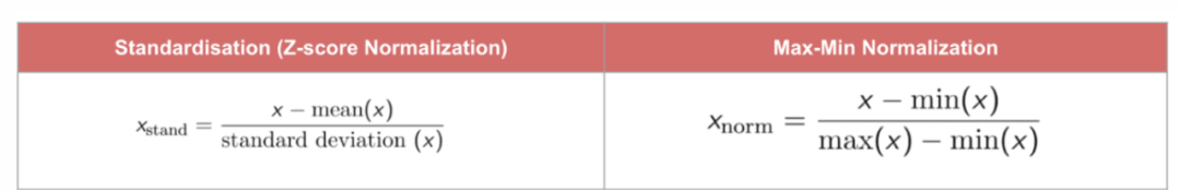
# Min-max normalization of training data
from sklearn.preprocessing import MinMaxScaler
sc = MinMaxScaler(feature_range = (0, 1))
training_set_scaled = sc.fit_transform(training_set)
Organize the data into samples and labels: 60 timesteps and 1 output
# Each sample contains 60 time steps, corresponding to the label value of the next time step
X_train = []
y_train = []
for i in range(60, 2035):
    X_train.append(training_set_scaled[i-60:i, 0])
    y_train.append(training_set_scaled[i, 0])
X_train, y_train = np.array(X_train), np.array(y_train)

print(X_train.shape)
print(y_train.shape)

# Reshaping
X_train = np.reshape(X_train, (X_train.shape[0], X_train.shape[1], 1))
print(X_train.shape)
Create a single hidden layer RNN model using Keras, and set the model optimization algorithm to Adam with the target function being the mean squared error (MSE)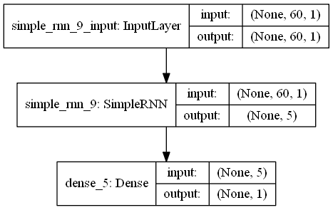
# Create RNN model using Keras

from keras.models import Sequential
from keras.layers import Dense
from keras.layers import SimpleRNN,LSTM
from keras.layers import Dropout


# Initialize sequential model
regressor = Sequential()

# Define input layer and hidden layer with 5 neurons
regressor.add(SimpleRNN(units = 5, input_shape = (X_train.shape[1], 1)))

# Define linear output layer
regressor.add(Dense(units = 1))

# Compile model: define optimization algorithm Adam, target function mean squared error
regressor.compile(optimizer = 'adam', loss = 'mean_squared_error')

# Model training
history = regressor.fit(X_train, y_train, epochs = 100, batch_size = 100, validation_split=0.1)

regressor.summary()
Display the model fitting situation: both the training set and validation set have low loss.
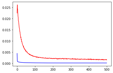
plt.plot(history.history['loss'],c='blue')    # Blue line for training set loss
plt.plot(history.history['val_loss'],c='red') # Red line for validation set loss
plt.show()
Evaluate the model: use a new time period of stock trading series data as the test set to assess the model’s performance on the test set.
# Test data
dataset_test = pd.read_csv('./data/tatatest.csv')
dataset_test = dataset_test.sort_values(by='Date').reset_index(drop=True)

real_stock_price = dataset_test.iloc[:, 1:2].values

dataset_total = pd.concat((dataset_train['Open'], dataset_test['Open']), axis = 0)
inputs = dataset_total[len(dataset_total) - len(dataset_test) - 60:].values
inputs = inputs.reshape(-1,1)
inputs = sc.transform(inputs)

# Extract test set
X_test = []
for i in range(60, 76):
    X_test.append(inputs[i-60:i, 0])
X_test = np.array(X_test)
X_test = np.reshape(X_test, (X_test.shape[0], X_test.shape[1], 1))

# Model prediction
predicted_stock_price = regressor.predict(X_test)
# Inverse normalization
predicted_stock_price = sc.inverse_transform(predicted_stock_price)
# Model evaluation
print('Prediction vs Actual MSE',sum(pow((predicted_stock_price - real_stock_price),2))/predicted_stock_price.shape[0])
print('Prediction vs Actual MAE',sum(abs(predicted_stock_price - real_stock_price))/predicted_stock_price.shape[0])
Through the test set evaluation, the prediction vs actual difference MSE: 53.03141531, prediction vs actual difference MAE: 5.82196445. Visualize the differences between predicted and actual values, which are overall quite consistent (Note: This article only predicts stock prices from the perspective of data patterns and does not constitute any investment advice; if you lose everything, don’t look for me  ).
).
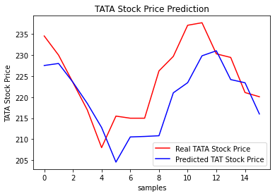
# Visualization of prediction vs actual differences
plt.plot(real_stock_price, color = 'red', label = 'Real TATA Stock Price')
plt.plot(predicted_stock_price, color = 'blue', label = 'Predicted TAT Stock Price')
plt.title('TATA Stock Price Prediction')
plt.xlabel('samples')
plt.ylabel('TATA Stock Price')
plt.legend()
plt.show()
– EOF –
1. Nüwa Algorithm, Crazy Kill!
2. This is the most serious software that China is stuck in!
3. Now I understand Convolutional Neural Networks (CNN)
If you find this article helpful, please share it with more people
Recommended to follow “Algorithm Enthusiasts”, to cultivate programming skills
Likes and views are the greatest support❤️