

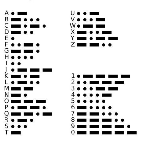
Warning: Actually, Morse code doesn’t need to be cracked. It is useful because messages can be sent with minimal equipment. The reason I say it doesn’t need to be cracked is that this code is well-known; the combination of dots and dashes is not a secret. But theoretically, it is a type of substitution cipher: each letter and each number is represented using dots and dashes, as shown in the figure below:
AI Frontline: Morse code is an intermittent signal code that expresses different English letters, numbers, and punctuation marks through different arrangements. It was invented in 1837. Morse code is an early form of digital communication, but unlike modern binary codes that only use two states of zero and one, its code includes five: dots, dashes, pauses between dots and dashes, medium pauses between words, and long pauses between sentences.
Let’s not doubt for now. Suppose we received a message in Morse code, but we don’t know how to interpret it. Let’s assume we have some code examples and their corresponding words. Now, we can infer that it is a type of substitution cipher, and we can ultimately calculate the code for each letter to decode the message.
Alternatively, we can build an encoder-decoder model to guess (almost) all the words! As masochists, we would certainly choose the latter. That said, let’s give a hearty pat to Don Quixote’s horse Rocinante and begin our journey to battle the windmills.
AI Frontline: Rocinante, in Spanish, means a rare steed. It is the name of the horse ridden by Don Quixote in the novel Don Quixote.
Here’s a pressing question: We have several encoded sequences and corresponding understandable examples. Using these examples, we must learn some patterns and use this information to predict what new encoded tokens (words) might be. Unlike common regression problems where we predict numerical outcomes, we have a sequence-to-sequence learning problem at hand, where the data has a temporal structure. This is an immediate hint that Recurrent Neural Networks (RNNs) might be useful (used for speech and voice data with RNNs, as well as for image data with CNNs and RNN combinations for image letters). Roughly speaking, this belongs to a class of problems that also includes machine translation; the structure of this model is inspirational here. For more information on this topic, please refer to [1]. Due to space constraints, we won’t elaborate on the theory of RNNs, but for a brief introduction to this topic, please refer to a series of articles in reference [2].
If you want to know whether this problem can be solved using different methods, the answer is: YES. The Markov Chain Monte Carlo (MCMC) method would yield similar results. In this case, we will follow the process mentioned in the first example from the excellent paper [3].
AI Frontline: The core idea of the Markov Chain Monte Carlo algorithm (abbreviated as MCMC) is to find a Markov chain of a certain state space such that the stable distribution of that Markov chain is our target distribution p(x). Thus, when we perform a random walk in that state space, the time spent in each state x is proportional to the target probability p(x). When sampling with MCMC, we first introduce an easily sampleable reference distribution q(x), and during each sampling step, we obtain a candidate sample y from q(x), and then decide whether to accept that sample according to certain principles; the determination of these principles ensures that the samples we obtain conform exactly to the p(x) distribution.
The Markov chain, named after Andrey Markov (A.A.Markov, 1856-1922), refers to a discrete event random process with the Markov property in mathematics. In this process, given the current knowledge or information, the past (i.e., the historical state before the current state) is irrelevant to predicting the future (i.e., the future state after the current state).
At each step of the Markov chain, the system can transition from one state to another based on a probability distribution or maintain its current state. The change of state is called a transition, and the probabilities associated with changing between different states are called transition probabilities. Random walks are an example of Markov chains. In a random walk, each step’s state is a point in a graph, and each step can move to any adjacent point, with the probability of moving to each point being the same (regardless of how the previous walk path was).
Roughly speaking, we want to predict the output sequence (y_1,…,y_m) from the input sequence (x_1,…,x_n), which involves learning conditional probabilities.
AI Frontline: Conditional probability refers to the probability of event A occurring given that event B has already occurred. Conditional probability is expressed as: P(A|B), read as “the probability of A given B.” Conditional probability can be calculated using decision trees. The fallacy of conditional probability assumes that P(A|B) is approximately equal to P(B|A).

The main obstacle here is predicting a variable-sized output from a variable-sized input. At the meta-level, this is addressed by combining two RNNs, where the first RNN maps variable-sized inputs to fixed-sized outputs, and the second RNN takes fixed-sized inputs and returns variable-sized outputs. The fixed-sized intermediate vector, called the context vector, encapsulates information from the input sequence, inputting one character at a time. The mechanism for generating the context vector makes RNNs useful for capturing temporal structures: the context vector is the final timestep or some function of its hidden state thereafter. The aforementioned conditional probability is computed using the chain rule.
AI Frontline: The chain rule is a differentiation rule in calculus used to find the derivative of a composite function. It is a commonly used method in calculus differentiation operations. The derivative of the composite function will be the product of the derivatives of the finite number of functions that make up the composite at the respective points, like a chain, hence the name chain rule. It is evident that mastering mathematics is crucial for doing AI.
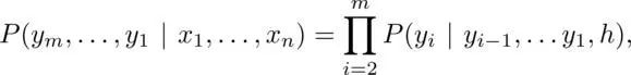
Here, h is the context vector. Finally, the softmax function can be used to calculate the conditional probability on the right side of the above equation, which takes the one-hot encoded vector of characters y_{i-1},…,y_1 as input, along with the outputs from the recurrent layer in the second RNN and the context vector. The specific type of RNN used here is LSTM, which effectively overcomes the limitations of Simple-RNN, which is affected by the vanishing gradient problem and can better capture long-range dependencies.
AI Frontline: Simple-RNN is the simplest form of recurrent neural network and serves as the foundation for LSTM. Like BP, Simple-RNN has both feedforward and feedback layers. However, Simple-RNN introduces a time (state)-based recurrent mechanism.
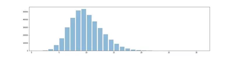
We will introduce a special character (11) to represent the spaces between the codes for each letter. For example, the code for SOS will be represented as: …11—*… (replacing …—…). We do this to ensure that the word corresponding to the given code is unique. Next, we will use English words from the compiled dataset (words_alpha) instead of a randomly generated letter set as our data. To get a feel for the data, refer to the histogram of word lengths shown below. From the histogram, it can be seen that words longer than 5 letters are more numerous than shorter words.
The networks trained on data containing encoded words generally predict longer words. Keep in mind that the network does not compute the “formula” that generates the data, meaning it does not learn the chart in Figure 1.
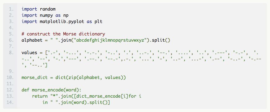
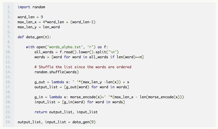
We begin the data preparation work by constructing a function that encodes the input English words into their Morse code and outputs it.
For illustrative purposes, we will generate training and validation data from a given fixed-length word. Here, we will fix this length to 9, as the number of words of length 9 is sufficiently large (see the histogram above). Note that this move means that the length of the output words from the network will be fixed, but the input Morse code does not necessarily have the same length. Assuming we know that the maximum encoding length for each letter is 4 (actually, we don’t need this specific assumption; we can choose the maximum length Morse code max_length_x to train the data). Therefore, if the length of the word is n, then the corresponding length of the Morse code can be at most 4n+(n-1), where n-1 corresponds to the number of 11s. We pad the codes with spaces on the left to make their lengths the same, which means our input character vocabulary is {‘.’, ‘—’, ‘*’, ‘ ’}. In general, we let the output character vocabulary be all letters and special characters for spaces. Returning to the comment about the network guessing long words, we mean that due to the number of long words causing an imbalance, the network will tend to guess fewer spaces. In the code snippet below, output_list will contain English words, and input_list will contain the padded Morse code.
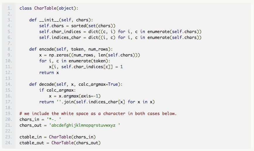
Now, we construct a one-hot encoded vector for the characters in the input, making the input data suitable for the neural network. To do this, we build a class object (similar to the example in the Keras documentation) that will help encode and decode Morse code and English words. We will assign the class to an object with the appropriate character set.
AI Frontline: One-hot encoding, also known as one-bit valid encoding, is a method that uses an N-bit state register to encode N states, with each state having its own independent register bit, and at any time, only one bit is valid.
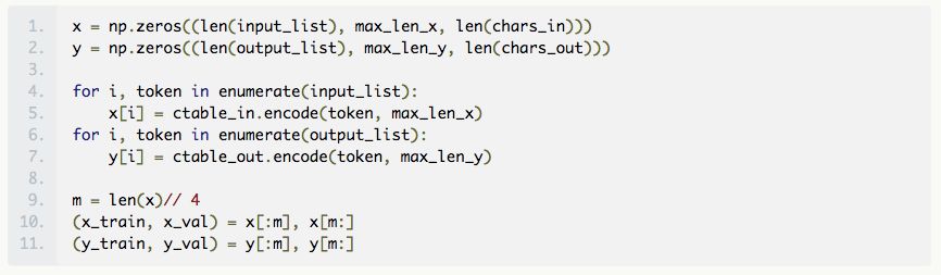
We split the data to generate a training set x_train, extracting y_train from one quarter of the entire dataset x, y, while retaining the remaining three-quarters as validation set x_val, y_val. Note that we should ideally set aside a portion of the training set as a validation set, with the remainder as a test set, but considering we are setting this up casually, we are more interested in model construction than parameter tuning. Now, we have prepared the training and testing (validation) data and can proceed to modify the network.
The simplest way to build a neural network is to use the Keras model and Sequential API. Since we do not need all the functionalities and flexibility of TensorFlow, we choose Keras.
The model topology we selected combines a powerful variant of simple RNNs called Long Short Term Memory (LSTM) networks.
AI Frontline: Long Short Term Memory networks are a type of time-based recurrent neural network suitable for handling and predicting important events with relatively long intervals and delays in time series. Systems based on Long Short Term Memory networks can perform tasks such as machine translation, video analysis, document summarization, speech recognition, image recognition, handwriting recognition, chatbot control, and music synthesis.
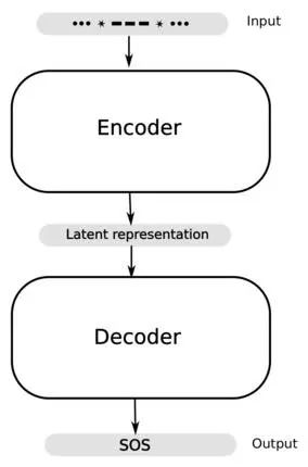
The first LSTM serves as the encoder, accepting a variable-length input sequence, one character at a time, and converting it into a fixed-length internal latent representation. Another LSTM acts as the decoder, taking the latent representation as input and passing its output to a dense layer that uses the softmax function to predict one character at a time.
The encoder and decoder components of the model may have multiple layers of LSTM, and it is generally unclear which topology is best to use. In general, deeper networks work better for machine translation. As a rule of thumb, we expect multiple layers to learn higher-level temporal representations, so we use them when the data has some hierarchical structure. For us, one layer is sufficient.
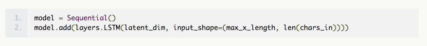
The model is built using Sequential() and adds one layer at a time. The first LSTM layer takes a 3D tensor as input and requires the user to specify the input dimensions. This can be easily done with the input_shape specified in the code, where the first component represents the number of timesteps, and the second component represents the number of features. For us, the number of features is the number of elements in the input sequence’s vocabulary, which is 4, as we have “.”, “-”, “*”, and the blank character “”. Since we provide a one-hot encoded vector each time, the number of timesteps is max_len_x. We will also specify the number of memory units (or blocks) in the layer (represented here by the latent_dim parameter, which we use as 256), which is the dimension of the latent representation. Note that we want to return the final hidden state of the LSTM as the latent representation, which contains information from all timesteps, i.e., the entire input sequence. If we use the return_sequences = true option, we will get outputs of hidden states for each timestep, but this only contains sequence information up to that timestep.
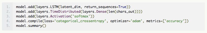
This results in a simple encoder model. We will build a similar layer as the decoder. However, the output of the code snippet above is a 2D array. We convert it to a 3D tensor by using the convenient RepeatVector layer to repeat the output timesteps max_len_y, which serves as the input for the next LSTM layer (the decoder). Now, we use the return_sequences = True option in this LSTM to output a sequence of hidden states, which we need for predictions. For this purpose, we use a TimeDistributed dense layer that outputs a vector of length max_len_y, using the softmax activation function to select the most likely letter. For a quick understanding of the purpose of the TimeDistributed layer, refer to the blog post by Jason Brownlee: How to Use the TimeDistributed Layer for Long Short-Term Memory Networks in Python.
https://machinelearningmastery.com/timedistributed-layer-for-long-short-term-memory-networks-in-python/
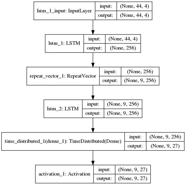
Below is a quick summary of the network and various input/output dimensions.
We will fit the model to the data, training on the sets x_train, y_train, and using x_val and y_val to check our work. The last set of parameters to set is the number of epochs and the batch size. The batch size is the size of the training set passed through the network in the gradient descent algorithm, after which the weights in the network are updated. Typically, the batch size is the maximum that the computer’s memory can handle. One epoch is a complete training of the training data through these batches once. Here, we set a batch size of 1024 and used 120 epochs; it can be seen from the figure below that after about 100 epochs, the accuracy did not significantly increase. Generally, it takes repeated experiments to see which parameters work. Now we use the fit() method to fit the model.

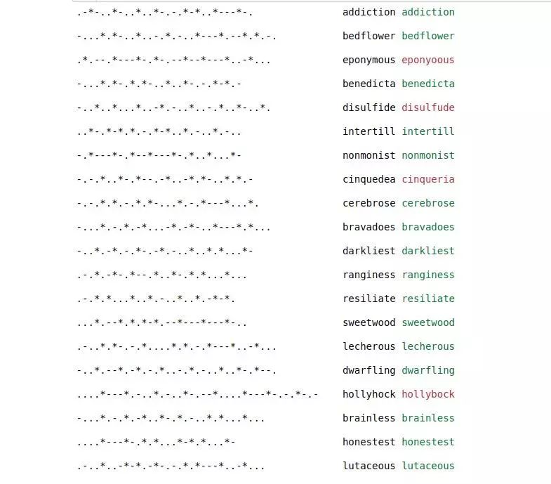
Finally, from the chart above, we can see that we can achieve about 93% accuracy on the validation set, and the results seem decent. Of course, we could do better if we increased the size of the training data. Below are predictions for a randomly selected set of words.

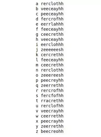
On the left, the input code; in the middle, the corresponding word; on the right, the prediction. If the prediction is correct, the word is green; otherwise, it is red.
As you can see, the incorrect predictions are not too bad. We must remind ourselves that deciphering a code does not mean cracking it, i.e., figuring out what each letter represents. In fact, we can input the letter codes and see the codes of individual letters predicted by the network, as shown below, and we are still far from the target!
As another example of an encoder-decoder model, you can try using the Caesar cipher or other codes to see how effective this method is.
AI Frontline: The Caesar cipher, also known as the Caesar shift, is one of the simplest and most well-known encryption techniques. It is a type of substitution cipher where all letters in the plaintext are replaced with letters some fixed number of positions down or up the alphabet. For example, with a shift of 3, all A’s would be replaced with D’s, B would become E, and so on. This encryption method is named after Caesar, who used it to communicate with his generals. The Caesar cipher is often used as a step in other, more complex encryption methods. The Caesar cipher is also applied in modern ROT13 systems. However, like all substitution-based encryption techniques, the Caesar cipher is very easy to crack and offers no guarantee of communication security in practical applications.
References:
[1] Sequence to Sequence Learning with Neural Networks
http://papers.nips.cc/paper/5346-sequence-to-sequence-learning-with-neural-networks.pdf
[2] Understanding LSTM Networks
http://colah.github.io/posts/2015-08-Understanding-LSTMs/
[3] THE MARKOV CHAIN MONTE CARLO REVOLUTION
http://www.ams.org/journals/bull/2009-46-02/S0273-0979-08-01238-X/S0273-0979-08-01238-X.pdf


If you want to see more articles like this, please give us a thumbs up!