Source: Deephub Imba


This article is approximately 2200 words long and is recommended for a 9-minute read. It includes an overview of its main classes and functions along with some code examples. It can serve as an introductory tutorial for this library.
Mainly includes Pipeline, Datasets, Metrics, and AutoClasses
Hugging Face is a very popular NLP library. This article includes an overview of its main classes and functions along with some code examples. It can serve as an introductory tutorial for this library.
Hugging Face is an open-source library for building, training, and deploying state-of-the-art NLP models. Hugging Face provides two main libraries: transformers for models and datasets for datasets. They can be installed directly using pip.
pip install transformers datasets
Pipeline
Using the Pipeline in the transformers library is the fastest and simplest way to start experimenting: simply provide a task name to the Pipeline object, and it will automatically download the appropriate model from the Hugging Face model repository!
The transformers library already provides the following tasks:
In addition, there are tasks related to computer vision and audio (mainly also based on transformers).
Below is an example of a sentiment analysis task. To predict the sentiment of a sentence, simply pass the sentence to the model.
from transformers import pipeline

classifier = pipeline("sentiment-analysis")

results = classifier("I'm so happy today!")
print(f"{results[0]['label']} with score {results[0]['score']}")
# POSITIVE with score 0.9998742341995239
The model’s output is a list of dictionaries, where each dictionary has a label (for this specific example, the value is ‘POSITIVE’ or ‘NEGATIVE’) and a score (i.e., the score of the predicted label).
You can provide multiple sentences to the classifier and get all results in a single function call.
results = classifier(["I'm so happy today!", "I hope you don't hate him..."])
for result in results:
  print(f"{result['label']} with score {result['score']}")
# POSITIVE with score 0.9998742341995239
# NEGATIVE with score 0.6760789155960083
You can also specify which model to use by setting the model name parameter. All models and information about the models are provided in the official documentation. For example, the code below uses twitter-roberta-base-sentiment.
classifier = pipeline("sentiment-analysis",
                    model="cardiffnlp/twitter-roberta-base-sentiment",
                    tokenizer="cardiffnlp/twitter-roberta-base-sentiment")
# three possible outputs:
# LABEL_0 -> negative
# LABEL_1 -> neutral
# LABEL_2 -> positive

results = classifier(["We are very happy to show you the 🤗 Transformers library.", "We hope you don't hate it."])
for result in results:
  print(f"{result['label']} with score {result['score']}")
# LABEL_2 with score 0.9814898371696472
# LABEL_1 with score 0.5063014030456543
Dataset
The Datasets library allows you to easily download some of the most common benchmark datasets used in NLP.
For example, to load the Stanford Sentiment Treebank (SST2), which aims for binary (positive and negative) classification with sentence-level labels, you can use the load_dataset function directly.
import datasets

dataset = datasets.load_dataset("glue", "sst2")

print(dataset)
DatasetDict({
  train: Dataset({
      features: ['sentence', 'label', 'idx'],
      num_rows: 67349
  })
  validation: Dataset({
      features: ['sentence', 'label', 'idx'],
      num_rows: 872
  })
  test: Dataset({
      features: ['sentence', 'label', 'idx'],
      num_rows: 1821
  })
})
The dataset has been divided into training, validation, and test sets. You can use the split parameter to call the load_dataset function and directly obtain the split of the dataset you are interested in.
dataset = datasets.load_dataset("glue", "sst2", split='train')

print(dataset)
Dataset({
  features: ['sentence', 'label', 'idx'],
  num_rows: 67349
})
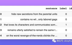
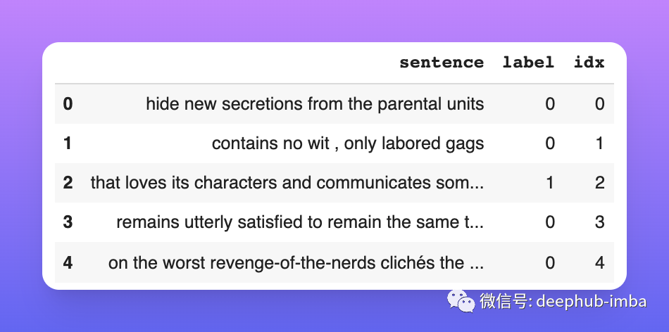
If you want to process the dataset using Pandas, you can create a DataFrame directly from the dataset object.
import pandas as pd

df = pd.DataFrame(dataset)
df.head()
Using GPU
Now that we have loaded a dataset for sentiment analysis, let’s start creating a sentiment analysis model.
First, let’s test predicting the sentiment of 500 sentences and measure how long it takes.
classifier = pipeline("sentiment-analysis")
%time results = classifier(dataset.data["sentence"].to_pylist()[:500])
# CPU times: user 21.9 s, sys: 56.9 ms, total: 22 s
# Wall time: 21.8 s
Predicting the sentiment of 500 sentences takes 21.8 seconds, averaging 23 sentences per second. Let’s try it on a GPU.
To make the classifier use a GPU, you must first ensure that the GPU is available, then use the parameter device=0. This way, the model can run on a CUDA-supported GPU, where each id from zero maps to a CUDA device, and the value -1 is for the CPU.
classifier = pipeline("sentiment-analysis", device=0)
%time results = classifier(dataset.data["sentence"].to_pylist()[:500])
# CPU times: user 4.07 s, sys: 49.6 ms, total: 4.12 s
# Wall time: 4.11 s
Predicting 500 sentences took only 4.1 seconds, averaging 122 sentences per second, improving speed by about 6 times! That’s right 😏
Metrics
If you want to test the quality of the classifier on the SST2 dataset, which metric should you use?
In Hugging Face, metrics and datasets are paired together. So you can call the load_metric function with the same parameters as load_dataset.
For the SST2 dataset, the metric is accuracy. You can directly obtain the metric value using the following code.
metric = datasets.load_metric("glue", "sst2")

n_samples = 500

X = dataset.data["sentence"].to_pylist()[:n_samples]
y = dataset.data["label"].to_pylist()[:n_samples]

results = classifier(X)
predictions = [0 if res["label"] == "NEGATIVE" else 1 for res in results]

print(metric.compute(predictions=predictions, references=y))
# {'accuracy': 0.988}
AutoClasses
The pipeline is implemented at a lower level by the AutoModel and AutoTokenizer classes. AutoClasses (such as AutoModel and AutoTokenizer) are shortcuts for loading models, which can automatically retrieve pre-trained models from their names or paths. When using them, you only need to choose the appropriate AutoModel for the task and use AutoTokenizer for its associated tokenizer: in this example, it is for text classification, so the correct AutoModel is AutoModelForSequenceClassification.
Now let’s see how to use AutoModelForSequenceClassification and AutoTokenizer to achieve the same functionality as the above Pipeline:
from transformers import AutoTokenizer, AutoModelForSequenceClassification

model_name = "nlptown/bert-base-multilingual-uncased-sentiment"
tokenizer = AutoTokenizer.from_pretrained(model_name)
model = AutoModelForSequenceClassification.from_pretrained(model_name)
Here, we create a tokenizer object using AutoTokenizer and a model object using AutoModelForSequenceClassification. You only need to pass the model’s name, and the rest will be done automatically.
Next, let’s see how to tokenize sentences using the tokenizer. The tokenizer output is a dictionary consisting of input_ids (the id of each token detected in the input sentence, taken from the tokenizer’s vocabulary), token_type_ids (used for models that require two texts for prediction, which we can ignore now), and attention_mask (indicating where padding occurred during tokenization).
encoding = tokenizer(["Hello!", "How are you?"], padding=True,
                    truncation=True, max_length=512, return_tensors="pt")

print(encoding)
{'input_ids': tensor([[ 101, 29155,   106,   102,     0,     0],
      [ 101, 12548, 10320, 10855,   136,   102]]), 'token_type_ids': tensor([[0, 0, 0, 0, 0, 0],
      [0, 0, 0, 0, 0, 0]]), 'attention_mask': tensor([[1, 1, 1, 1, 0, 0],
      [1, 1, 1, 1, 1, 1]])}
Then pass the tokenized sentences to the model, which is responsible for outputting predictions. This specific model outputs five scores, where each score is the probability of the rating from 1 to 5.
outputs = model(**encoding)

print(outputs)
SequenceClassifierOutput(loss=None, logits=tensor([[ -0.2410, -0.9115, -0.3269, -0.0462, 1.2899],
      [ -0.3575, -0.6521, -0.4409, 0.0471, 0.9552]],
      grad_fn=<AddmmBackward0>), hidden_states=None, attentions=None)
The model outputs the final results in the logits attribute. Applying the softmax function to the logits can obtain the probabilities for each label.
from torch import nn

pt_predictions = nn.functional.softmax(outputs.logits, dim=-1)

print(pt_predictions)
tensor([[0.1210, 0.0619, 0.1110, 0.1470, 0.5592],
      [0.1269, 0.0945, 0.1168, 0.1902, 0.4716]], grad_fn=<SoftmaxBackward0>)
Saving and Loading Models Locally
Finally, let’s see how to save a model locally. This can be done using the save_pretrained function of the tokenizer and model.
pt_save_directory = "./model"
tokenizer.save_pretrained(pt_save_directory)
model.save_pretrained(pt_save_directory)
If you want to load a model that was previously saved, you can use the from_pretrained function of the AutoModel class to load it.
model = AutoModelForSequenceClassification.from_pretrained("./model")
Conclusion
This article introduced the main classes and functions of the Hugging Face library, including the datasets library of transformers, how to use Pipeline to load models in just a few lines of code, and how to run this code on CPU or GPU. It also introduced how to load benchmark datasets directly from the library and how to compute metrics. Finally, it demonstrated how to use the two most important classes, AutoModel and AutoTokenizer, and how to save and load models locally. With this introduction, I hope you can start your NLP journey using the Hugging Face library.