
Source: Turing Artificial Intelligence
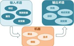
Depending on the type of data, modeling a problem can be approached in different ways. In the field of machine learning or artificial intelligence, people first consider the learning method of the algorithm. There are several main learning methods in machine learning. Categorizing algorithms according to their learning methods is a good idea, as it allows people to consider the most suitable algorithm based on the input data when modeling and selecting algorithms to achieve the best results.

1. Supervised Learning:
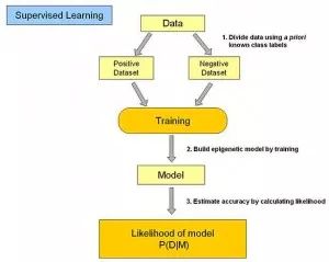
In supervised learning, the input data is referred to as “training data”, and each set of training data has a clear label or result, such as “spam” or “not spam” in a spam detection system, or “1”, “2”, “3”, “4”, etc., in handwritten digit recognition. When building a predictive model, supervised learning establishes a learning process that compares the predicted results with the actual results of the “training data” and continuously adjusts the predictive model until the model’s predictions reach an expected accuracy rate. Common applications of supervised learning include classification problems and regression problems. Common algorithms include Logistic Regression and Back Propagation Neural Network.
2. Unsupervised Learning:

In unsupervised learning, the data is not specially labeled, and the learning model is designed to infer some intrinsic structure of the data. Common application scenarios include learning association rules and clustering. Common algorithms include Apriori Algorithm and k-Means Algorithm.
3. Semi-Supervised Learning:
In this learning method, part of the input data is labeled while part is not. This learning model can be used for predictions, but the model first needs to learn the intrinsic structure of the data to organize it reasonably for predictions. Application scenarios include classification and regression, and algorithms include extensions of commonly used supervised learning algorithms that first attempt to model the unlabeled data and then predict the labeled data based on that. Examples include Graph Inference Algorithm or Laplacian SVM.
4. Reinforcement Learning:
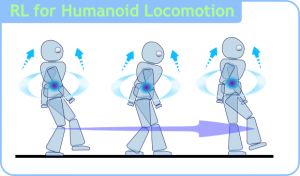
In this learning mode, the input data serves as feedback to the model. Unlike supervised models where the input data is merely a way to check the correctness of the model, in reinforcement learning, the input data directly feeds back to the model, which must make immediate adjustments. Common application scenarios include dynamic systems and robot control. Common algorithms include Q-Learning and Temporal Difference Learning.
In the context of enterprise data applications, the most commonly used models are likely supervised and unsupervised learning. In fields like image recognition, where there is a large amount of unlabeled data and a small amount of labeled data, semi-supervised learning is currently a hot topic. Reinforcement learning is more commonly applied in robot control and other fields requiring system control.
5. Algorithm Similarity
Based on the similarity of the functions and forms of algorithms, we can classify algorithms, such as tree-based algorithms, neural network-based algorithms, etc. Of course, the scope of machine learning is vast, and some algorithms are difficult to clearly categorize into one type. For some classifications, algorithms within the same category can target different types of problems. Here, we try to classify commonly used algorithms in the most understandable way.
6. Regression Algorithms:
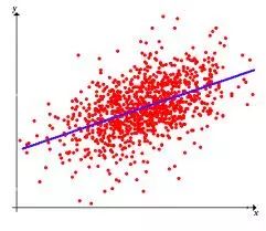
Regression algorithms attempt to explore the relationships between variables by measuring errors. Regression algorithms are powerful tools in statistical machine learning. In the field of machine learning, when people mention regression, it sometimes refers to a type of problem and sometimes to a type of algorithm, which often confuses beginners. Common regression algorithms include Ordinary Least Square, Logistic Regression, Stepwise Regression, Multivariate Adaptive Regression Splines, and Locally Estimated Scatterplot Smoothing.
7. Instance-Based Algorithms
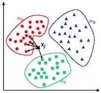
Instance-based algorithms are often used to build models for decision-making problems. These models typically first select a batch of sample data and then compare new data with the sample data based on certain similarities. This approach is used to find the best match. Therefore, instance-based algorithms are also known as “winner-takes-all” learning or “memory-based learning”. Common algorithms include k-Nearest Neighbor (KNN), Learning Vector Quantization (LVQ), and Self-Organizing Map (SOM).
8. Regularization Methods
Regularization methods extend other algorithms (usually regression algorithms) by adjusting them based on algorithm complexity. Regularization methods typically reward simpler models while penalizing complex algorithms. Common algorithms include Ridge Regression, Least Absolute Shrinkage and Selection Operator (LASSO), and Elastic Net.
9. Decision Tree Learning
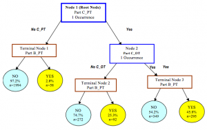
Decision tree algorithms use a tree structure to establish decision models based on data attributes. Decision tree models are often used to solve classification and regression problems. Common algorithms include Classification And Regression Tree (CART), ID3 (Iterative Dichotomiser 3), C4.5, Chi-squared Automatic Interaction Detection (CHAID), Decision Stump, Random Forest, Multivariate Adaptive Regression Splines (MARS), and Gradient Boosting Machine (GBM).
10. Bayesian Methods

Bayesian method algorithms are a class of algorithms based on Bayes’ theorem, mainly used to solve classification and regression problems. Common algorithms include Naive Bayes, Averaged One-Dependence Estimators (AODE), and Bayesian Belief Network (BBN).
11. Kernel-Based Algorithms
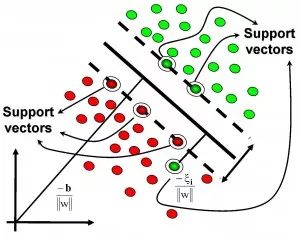
The most famous kernel-based algorithm is the Support Vector Machine (SVM). Kernel-based algorithms map input data to a higher-dimensional vector space, where some classification or regression problems can be more easily solved. Common kernel-based algorithms include Support Vector Machine (SVM), Radial Basis Function (RBF), and Linear Discriminant Analysis (LDA).
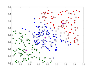
12. Clustering Algorithms

Clustering, like regression, sometimes refers to a class of problems and sometimes to a class of algorithms. Clustering algorithms usually merge input data based on centroids or hierarchical methods. All clustering algorithms attempt to find the intrinsic structure of the data in order to classify it based on the greatest commonalities. Common clustering algorithms include k-Means Algorithm and Expectation Maximization (EM).
13. Association Rule Learning
Association rule learning seeks to find the rules that best explain the relationships between data variables, identifying useful association rules in large multi-dimensional datasets. Common algorithms include Apriori Algorithm and Eclat Algorithm.
14. Artificial Neural Networks
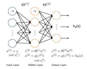
Artificial neural network algorithms simulate biological neural networks and are a class of pattern matching algorithms. They are typically used to solve classification and regression problems. Artificial neural networks represent a huge branch of machine learning, with hundreds of different algorithms (including deep learning, which will be discussed separately). Important artificial neural network algorithms include Perceptron Neural Network, Back Propagation, Hopfield Network, Self-Organizing Map (SOM), and Learning Vector Quantization (LVQ).
15. Deep Learning
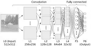
Deep learning algorithms represent an evolution of artificial neural networks. Recently, they have gained a lot of attention, especially after Baidu began to focus on deep learning, which has drawn significant attention domestically. As computational power becomes increasingly affordable, deep learning aims to establish much larger and more complex neural networks. Many deep learning algorithms are semi-supervised learning algorithms designed to handle large datasets with a small amount of unlabeled data. Common deep learning algorithms include Restricted Boltzmann Machine (RBM), Deep Belief Networks (DBN), Convolutional Networks, and Stacked Auto-encoders.
16. Dimensionality Reduction Algorithms

Like clustering algorithms, dimensionality reduction algorithms attempt to analyze the intrinsic structure of the data, but they do so in an unsupervised manner, trying to summarize or explain data using less information. These algorithms can be used for visualizing high-dimensional data or simplifying data for supervised learning use. Common algorithms include Principal Component Analysis (PCA), Partial Least Square Regression (PLS), Sammon Mapping, Multi-Dimensional Scaling (MDS), and Projection Pursuit.
17. Ensemble Algorithms:

Ensemble algorithms train several relatively weak learning models independently on the same samples and then combine the results for overall predictions. The main challenge of ensemble algorithms lies in determining which independent weak learning models to combine and how to integrate the learning results. This is a very powerful and popular class of algorithms. Common algorithms include Boosting, Bootstrapped Aggregation (Bagging), AdaBoost, Stacked Generalization (Blending), Gradient Boosting Machine (GBM), and Random Forest.
Common advantages and disadvantages of machine learning algorithms:
Naive Bayes:
1. If the length of the given feature vector may vary, it needs to be normalized to a common length vector (for example, in text classification, if it is a sentence of words, the length is equal to the total vocabulary length, with corresponding positions being the count of occurrences of that word).
2. The calculation formula is as follows:
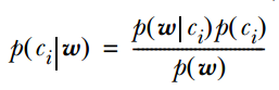
One of the conditional probabilities can be expanded using the naive Bayes conditional independence assumption. It is important to note that  is calculated, and based on the naive Bayes assumption,
 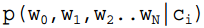 =
= , hence generally there are two methods: one is to find the total occurrences of wj in the samples of class ci and divide it by the total of that sample; the second method is to find the total occurrences of wj in the samples of class ci and divide it by the total occurrences of all features in that sample.
3. If any item in  is 0, the product of the joint probabilities may also be 0, meaning the numerator of the formula in 2 is 0. To avoid this, one generally initializes this item to 1; of course, to ensure equal probabilities, the denominator should correspondingly be initialized to 2 (since there are 2 classes, if there are k classes, k should be added, a technique known as Laplace smoothing, where the denominator is increased by k to satisfy the total probability formula).
The advantages of naive Bayes are its good performance on small-scale data, suitability for multi-class tasks, and suitability for incremental training.
Disadvantages: it is sensitive to the expression form of input data.
Decision Trees: An important aspect of decision trees is selecting an attribute for branching, so attention should be paid to the calculation formula for information gain and its deep understanding.
The calculation formula for information entropy is as follows:
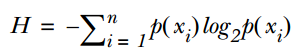
Where n represents the number of classification categories (for example, if it is a binary classification problem, then n=2). Calculate the probabilities p1 and p2 of these two categories in the total samples, allowing us to compute the information entropy before selecting an attribute for branching.
Now, if we select an attribute xi for branching, the branching rule is: if xi=vx, the sample goes to one branch of the tree; if not, it goes to the other branch. It is evident that the samples in the branches likely include two categories, so we calculate the entropies H1 and H2 for these two branches, calculating the total information entropy after branching as H’=p1*H1+p2*H2. The information gain at this point is ΔH=H-H’. Using information gain as the principle, we test all attributes and select the one that maximizes the gain as the branching attribute for this round.
The advantages of decision trees include simple calculations, strong interpretability, suitability for handling samples with missing attribute values, and the ability to handle irrelevant features.
Disadvantages: they are prone to overfitting (subsequent methods like Random Forest have reduced overfitting).
Logistic Regression: Logistic is used for classification and is a type of linear classifier. Important points to note include:
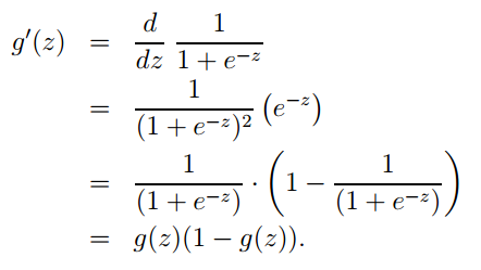
1. The logistic function expression is:
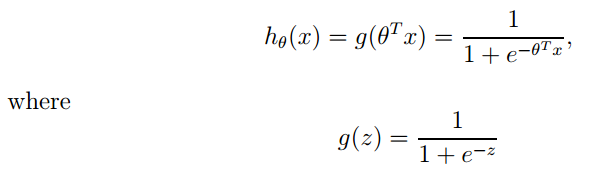
Its derivative form is:
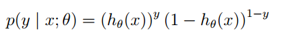
2. The logistic regression method mainly learns using maximum likelihood estimation, so the posterior probability of a single sample is:
For the posterior probability of the entire sample:
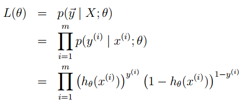
Where:

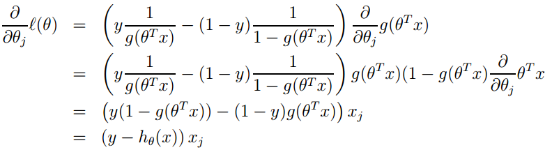
By further simplifying using logarithms:
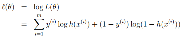
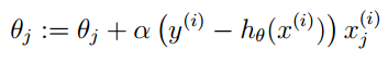
3. Its loss function is -l(θ), so we need to minimize the loss function, which can be achieved using gradient descent. The gradient descent formula is:
The advantages of logistic regression include:
1. Simple implementation.
2. Very low computational load during classification, fast speed, and low storage resource usage.
Disadvantages:
1. Prone to underfitting, generally low accuracy.
2. Can only handle binary classification problems (Softmax, derived from this, can be used for multi-class classification) and must be linearly separable.
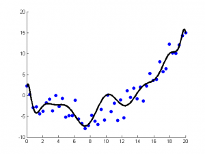
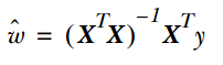
Linear Regression: Linear regression is truly used for regression, unlike logistic regression, which is used for classification. Its basic idea is to optimize the error function in the form of least squares using gradient descent, and it can also directly solve for the parameters using the normal equation, resulting in:
In LWLR (Locally Weighted Linear Regression), the parameter calculation expression is:
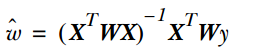
Because at this time, the optimization is:
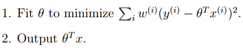
It can be seen that LWLR differs from LR in that LWLR is a non-parametric model because each regression calculation must traverse the training samples at least once.
The advantages of linear regression include simple implementation and simple calculations.
Disadvantages: cannot fit non-linear data.
KNN Algorithm: KNN, or k-nearest neighbors, primarily involves the following steps:
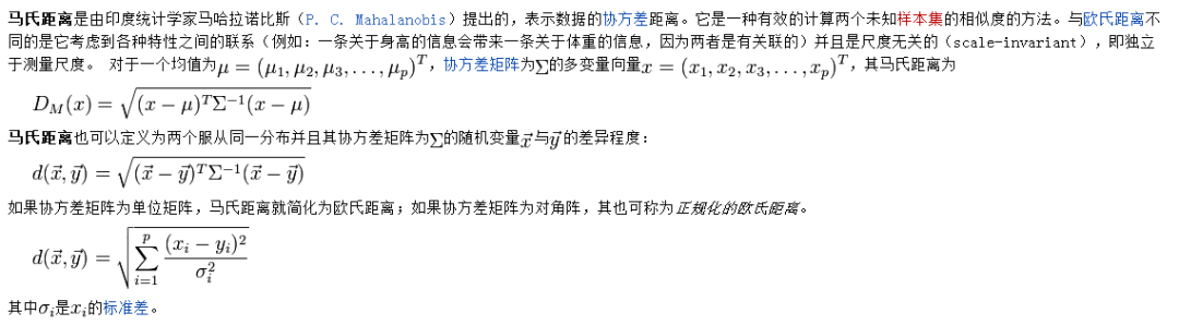
1. Calculate the distance between each sample point in the training samples and the test samples (common distance metrics include Euclidean distance, Mahalanobis distance, etc.);
2. Sort all the distance values obtained above;
3. Select the top k samples with the smallest distances;
4. Based on the labels of these k samples, perform voting to obtain the final classification category;
Choosing the best K value depends on the data. Generally, a larger K value can reduce the impact of noise but can make the boundaries between categories blurrier. A good K value can be obtained through various heuristic techniques, such as cross-validation. Additionally, the presence of noise and irrelevant feature vectors can reduce the accuracy of the K-nearest neighbors algorithm.
The KNN algorithm has strong consistency results. As the data approaches infinity, the algorithm ensures that the error rate does not exceed twice that of the Bayesian algorithm’s error rate. For some good K values, KNN guarantees that the error rate does not exceed that of the Bayesian theoretical error rate.
Note: The Mahalanobis distance must first provide the statistical properties of the sample set, such as mean vector, covariance matrix, etc. An introduction to Mahalanobis distance is as follows:
The advantages of the KNN algorithm include:
1. Simple concept, mature theory, can be used for both classification and regression;
2. Can handle non-linear classification;
3. Training time complexity is O(n);
4. High accuracy, no assumptions about the data, and insensitivity to outliers;
Disadvantages:
1. High computational load;
2. Sample imbalance problem (i.e., some categories have many samples, while others have very few);
3. Requires a large amount of memory;
SVM: You need to learn how to use libsvm and some parameter tuning experiences, and also clarify some ideas of the SVM algorithm:
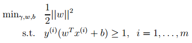
1. The optimal classification surface in SVM maximizes the geometric margin for all samples (to explain why the maximum margin classifier is chosen, please explain from a mathematical perspective; this was asked during an interview for a deep learning position at NetEase. The answer is that there is a relationship between geometric margin and the number of misclassifications: 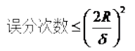 , where the denominator is the distance from the sample to the classification margin, and R is the longest vector value among all samples), thus:
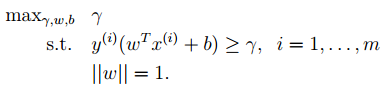
Through a series of derivations, we obtain the following original optimization target:
2. Next, let’s look at Lagrange theory:
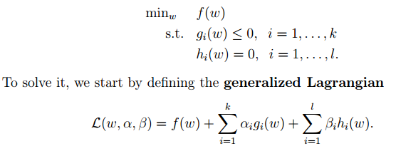
We can convert the optimization target in 1 into the form of Lagrange (through various dual optimizations and KKT conditions), and the final objective function is:
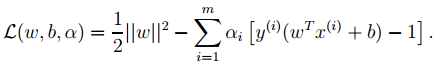
We only need to minimize the objective function above, where α is the Lagrange multiplier associated with the inequality constraints in the original optimization problem.
3. By taking derivatives of the last expression in 2 with respect to w and b, we can obtain:
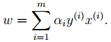
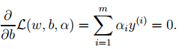
From the first expression above, we can see that if we optimize α, we can directly derive w, thus completing the model parameters. The second expression can serve as a constraint for subsequent optimization.
4. The last objective function in 2 can be transformed into the optimization of the following objective function using dual optimization theory:
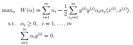
This function can be solved for α using common optimization methods, and then w and b can be derived.
5. Theoretically, the simple theory of SVM should end here. However, it is worth adding that during prediction:
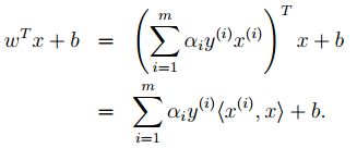
The angle brackets can be replaced with kernel functions, which is why SVM is often associated with kernel functions.
6. Finally, regarding the introduction of slack variables, the original optimization formula becomes:
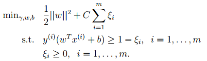
The corresponding dual optimization formula becomes:
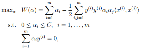
Compared to the previous one, α simply has an upper bound.
The advantages of SVM include:
1. Can be used for linear/non-linear classification and regression;
2. Low generalization error;
3. Easy to interpret;
4. Low computational complexity;
Disadvantages:
1. Sensitive to parameter and kernel function selection;
2. The original SVM is primarily adept at handling binary classification problems;
Boosting:
Using Adaboost as an example, let’s first look at the flowchart of Adaboost:
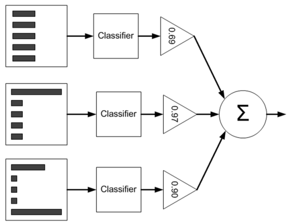
From the diagram, we can see that during training, we need to train multiple weak classifiers (3 in the diagram), each weak classifier is trained using samples with different weights (5 training samples in the diagram), while each weak classifier contributes differently to the final classification result, which is output through a weighted average. The weights are shown in the numbers inside the triangle in the diagram. So how are these weak classifiers and their corresponding weights trained?
Let’s explain this through a simple example, assuming we have 5 training samples, each with a dimension of 2. In training the first classifier, the weights for the 5 samples are all 0.2. Note that the sample weights and the weights α corresponding to the final trained weak classifier are different; the sample weights are only used during training, while α is used during both training and testing.
Now assume that the weak classifier is a simple decision tree with one node that selects one of the two attributes (assuming there are only two attributes) and computes the optimal value of that attribute for classification.
The training process of the simple version of Adaboost is as follows:
1. Train the first classifier, with the sample weights D being equal. Using a weak classifier, we get the predicted labels for these 5 samples (please refer to the example in the book, still Machine Learning in Action), comparing them with the true labels may result in errors (i.e., mistakes). If a sample is predicted incorrectly, its error value is its weight; if classified correctly, the error value is 0. Finally, the sum of the error rates for the 5 samples is denoted as ε.
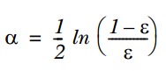
2. Using ε to calculate the weight α for the weak classifier, the formula is as follows:
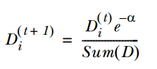
3. Using α to calculate the weights D for the next weak classifier, if a corresponding sample is classified correctly, its weight decreases, according to the formula:

If a sample is classified incorrectly, its weight increases, according to the formula:
4. Repeat steps 1, 2, and 3 to continue training multiple classifiers, just with different D values.
The testing process is as follows:
Input a sample into each of the trained weak classifiers, then each weak classifier corresponds to an output label, and the label is multiplied by the corresponding α. Finally, summing these values gives the sign as the predicted label.
The advantages of the boosting algorithm include:
1. Low generalization error;
2. Easy to implement, high classification accuracy, with few parameters to tune;
3. Disadvantages:
4. Sensitive to outliers;
Clustering:
Based on clustering ideas, the main reason is that in anomaly detection, the number of abnormal samples is very small while the number of normal samples is very large, making it insufficient to learn good parameters for the anomaly behavior model, as the incoming abnormal samples may completely differ from the patterns in the training samples.
EM Algorithm: Sometimes, because the generation of samples is related to latent variables (which cannot be observed), the parameters of the model are generally estimated using maximum likelihood. Due to the presence of latent variables, it is impossible to derive the likelihood function parameters; the EM algorithm can be used to estimate the model parameters (which may involve multiple parameters).
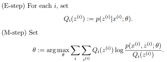
The EM algorithm generally consists of two steps:
E-step: Select a set of parameters and compute the conditional probability of the latent variables under these parameters;
M-step: Combine the conditional probabilities of the latent variables obtained in the E-step to maximize the lower bound of the likelihood function (essentially a certain expected function).
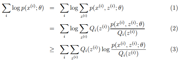
Repeat the above two steps until convergence, as shown in the formula:
The derivation process of the lower bound function in the M-step is:
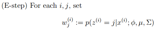
A common example of the EM algorithm is the GMM model, where each sample may be generated by k Gaussians, with different probabilities for each Gaussian. Thus, each sample corresponds to a Gaussian distribution (one of the k), and the latent variable is the Gaussian distribution corresponding to each sample.
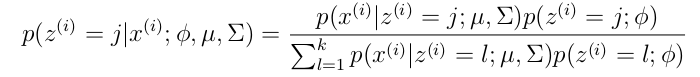
The E-step formula for GMM is as follows (calculating the probability of each sample corresponding to each Gaussian):
The more specific calculation formula is:
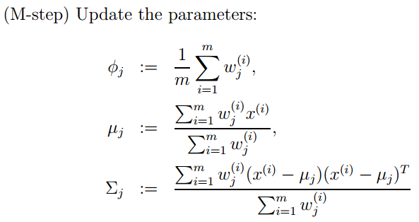
The M-step formula is as follows (calculating the weights, means, and variances of each Gaussian):
Apriori is one of the earlier methods in association analysis, mainly used to mine frequent itemsets. Its ideas are:
1. If an itemset is not frequent, then any superset containing it cannot be frequent;
2. If an itemset is frequent, then any non-empty subset of it is also frequent.
Apriori requires multiple scans of the item table, starting from one item and scanning, discarding those that are not frequent, yielding a set called L. Then, for each element in L, self-combination is performed to generate a set with one more item than the last scan, called C, and then scanning again to discard non-frequent items, repeating this process.
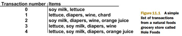
See the following example of an item table:
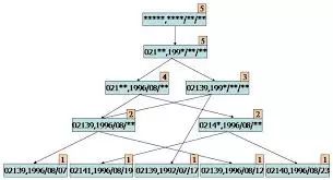
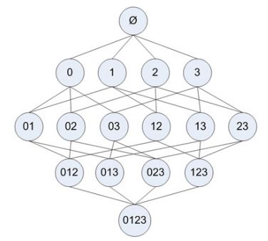
If at each step non-frequent itemsets are not discarded, the scanning process tree structure is as follows:
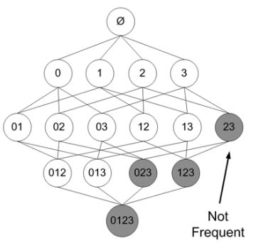
In one of the processes, if a non-frequent itemset appears, discarding it (indicated in shadow) results in:
FP Growth is a more efficient frequent item mining method than Apriori, requiring only two scans of the item table. The first scan obtains the frequency of each item, discarding those that do not meet support requirements, and sorting the remaining items. The second scan builds a FP-Tree (frequent-pattern tree).
The subsequent work involves mining on the FP-Tree; for example, the following table:
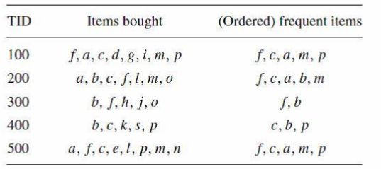
Corresponds to the FP_Tree as follows:
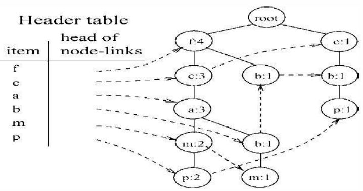
Then, starting from the least frequent single item P, find the conditional pattern base for P, constructing the FP_Tree for the conditional pattern base of P in the same way, and identifying the frequent itemsets containing P on this tree.
Sequentially mining frequent itemsets from the conditional pattern bases of m, b, a, c, f, some items require recursive mining, which can be quite cumbersome, such as for the m node.
This is for academic sharing only, copyright belongs to the original author.
How to Join the Society
Register as a Society Member:
Individual Membership:
Follow the Society’s WeChat: Follow the Society’s WeChat: China Command and Control Society (c2_china), reply “Individual Member” to obtain the membership application form, fill it out as required, and if there are any questions, you can leave a message in the public account. You can pay the membership fee online through Alipay after the society’s review.
Unit Membership:
Follow the Society’s WeChat: China Command and Control Society (c2_china), reply “Unit Member” to obtain the membership application form, fill it out as required, and for any questions, you can leave a message in the public account. You can pay the membership fee after the society’s review.
Long press the QR code below to follow the Society’s WeChat