Author: Andrey Kurenkov
As the puzzle of training multi-layer neural networks is unraveled, this topic has once again become extraordinarily popular, and Rosenblatt’s lofty ambitions seem to be realized. Until 1989, another key discovery was published, which is still widely cited in textbooks and major lectures.
Multi-layer feedforward neural networks are universal approximators. Essentially, it can be mathematically proven that the multi-layer structure allows neural networks to theoretically perform any function representation, including the XOR problem.
However, this is mathematics; you can imagine having infinite memory and the required computational power in mathematics—can backpropagation allow neural networks to be used in any corner of the world? Oh, certainly. Also in 1989, Yann LeCun validated an outstanding application of backpropagation in the real world at AT&T Bell Labs, namely “Backpropagation Applied to Handwritten Zip Code Recognition.”
You might think that enabling computers to correctly understand handwritten digits is not that impressive, and today it may seem overly dramatic, but in fact, before this application was publicly released, human handwriting was chaotic, and the disjointed strokes posed a great challenge to the computer’s uniform way of thinking. This study used a large amount of data from the United States Postal Service and demonstrated that neural networks could fully handle recognition tasks. More importantly, this study emphasized the practical need to move beyond plain backpropagation to a key transition towards modern deep learning.
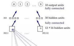
Traditional visual pattern recognition work has proven advantageous by extracting local features and combining them to form higher-level features. By forcing hidden units to combine local information sources, such knowledge can be easily structured into a network. The essential features of an object can appear at different positions in the input image. Therefore, having a set of feature detectors that can detect a specific feature instance located anywhere in the input stage is very wise. Since the precise location of a feature is irrelevant to classification, we can appropriately discard some location information during processing. However, approximate location information must be retained to allow the subsequent network layer to detect more advanced and complex features. (Fukushima1980, Mozer,1987)
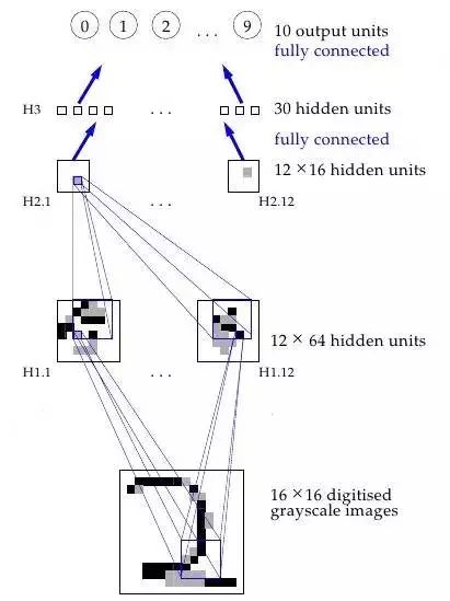
A visualization process of how a neural network works
Or, more specifically: the first hidden layer of a neural network is the convolutional layer—unlike traditional network layers, each neuron corresponds to a pixel in the image, each having a different weight (40*60=2400 weights), and only a small portion of the weights (5*5=25) is applied to a small complete subspace of the image of the same size. So, for example, instead of using four different neurons to learn to detect the 45-degree diagonals of the four corners of the entire input image, a single neuron can learn to detect the 45-degree diagonal in the subspace of the image and learn the entire image in this manner. The first process of each layer operates in a similar way, but receives the “local” feature positions found in the previous hidden layer rather than the pixel values of the image. Moreover, since they are combining information about the increasingly larger subsets of the image, they can also “see” the remaining larger parts of the image. Finally, the last two network layers utilize the more advanced and prominent features abstracted from the previous convolution to determine where the input image should be classified. This method proposed in the 1989 paper continues to serve as the foundation for the nationwide check reading systems.
Why does this work? The reason is intuitive, if the mathematical expression is not so clear: without these constraints, the network would have to learn the same simple things (like detecting straight lines at 45° angles and small circles, etc.) and would take a lot of time to learn every part of the image. However, with some constraints, each simple feature only needs one neuron to learn—and due to the significant reduction in overall weights, the entire process is completed faster. Moreover, since the precise location of these features is irrelevant, it can essentially skip over adjacent subsets of the image—subset sampling, a type of pooling—when applying weights, further reducing training time. Adding these two layers—the convolutional layer and the pooling layer—is the main distinction between convolutional neural networks (CNNs/ConvNets) and ordinary old neural networks.

The operational process of Convolutional Neural Networks (CNN)
At that time, the idea of convolution was referred to as “weight sharing,” which was also practically discussed in the 1986 extension analysis of backpropagation by Rumelhart, Hinton, and Williams. Clearly, Minsky and Papert’s analysis in the 1969 “Perceptrons” could raise questions that stimulated this research idea. However, as before, others had independently researched it—such as Kunihiko Fukushima’s Neurocognitron proposed in 1980. Moreover, as before, this idea drew inspiration from brain research:
According to Hubel and Wiesel’s hierarchical model, neural networks in the visual cortex have a hierarchical structure: LGB (lateral geniculate body) → simple cells → complex cells → low-order hyper-complex cells → high-order hyper-complex cells. The neural network between low-order hyper-complex cells and high-order hyper-complex cells has a structure similar to that between simple cells and complex cells. In this layered structure, higher-level cells tend to selectively respond to more complex features of stimulus patterns, while also having a larger receptive field and being less sensitive to the movement of stimulus pattern locations. Thus, a structure similar to the hierarchical model is introduced into our model.
LeCun also continued to support convolutional neural networks at Bell Labs, and his corresponding research results were ultimately successfully applied to check reading in the mid-1990s—his talks and interviews often introduced this fact: “In the late 1990s, one of these systems read about 10% to 20% of the checks in the United States.”
Neural Networks Entering the Era of Unsupervised Learning
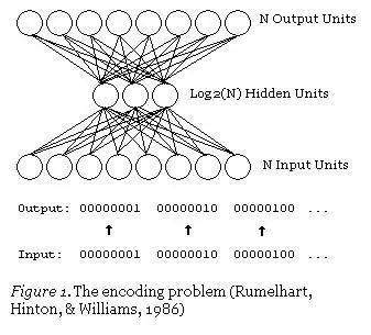
Automating the tedious and completely uninteresting task of check reading is an example of machine learning’s grand display. Perhaps there’s a predictive little application? Compression. This refers to finding a more compact representation of data and recovering the original representation from it; the compression methods found through machine learning may surpass all existing compression patterns. Of course, this means finding a smaller representation of the data from which the original data can be reconstructed. Learning this compression scheme far exceeds conventional compression algorithms, as the learning algorithm can find data features that might be missed under conventional compression algorithms. Moreover, this is easy to do—just train a neural network with a small hidden layer to output the input.
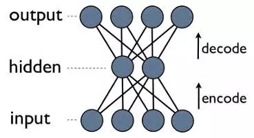
Autoencoder Neural Networks
This is an autoencoder neural network, which is also a method of learning compression—effectively transforming data into a compressed format and automatically returning to itself. We can see that the output layer calculates its output. Since the output of the hidden layer is less than that of the input layer, the output of the hidden layer is a compressed expression of the input data, which can be reconstructed at the output layer.
Understanding Autoencoder Compression More Clearly
Notice something wonderful: the only thing we need for training is some input data. This sharply contrasts with the requirements of supervised machine learning, which requires a training set of input-output pairs (labeled data) to approximately generate a function that can produce corresponding outputs from these inputs. Indeed, autoencoders are not a form of supervised learning; they are actually a form of unsupervised learning that only requires a set of input data (unlabeled data) with the goal of finding some hidden structure within that data. In other words, unsupervised learning is less about approximating functions and more about generating another useful representation from input data. This representation can reconstruct better than the original data, but it can also be used to find similar data groups (clustering) or infer other latent variables (some aspects that appear to exist from the data but are numerically unknown).
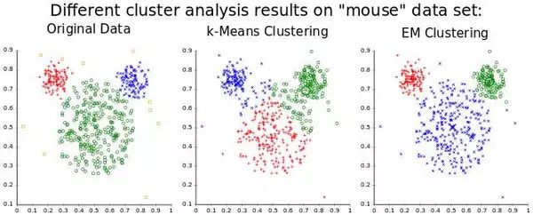
Clustering, a very common application of unsupervised learning
Before and after the discovery of the backpropagation algorithm, neural networks had other unsupervised applications, the most famous of which are self-organizing map neural networks (SOM) and adaptive resonance theory (ART). SOM can generate low-dimensional data representations for easier visualization, while ART can learn to classify arbitrary input data without being told the correct categories. If you think about it, it is intuitive that a lot can be learned from unlabeled data. Suppose you have a dataset containing a bunch of handwritten digits, without labeling which digit corresponds to each image. If an image contains a digit from the dataset, it looks similar to most other images with the same digit. Thus, even though the computer may not know which digit corresponds to these images, it should be able to discover that they all correspond to the same digit. Thus, pattern recognition is the task that most machine learning aims to solve and may also be the basis of the human brain’s powerful abilities. However, let us not deviate from our journey into deep learning; let’s return to autoencoders.
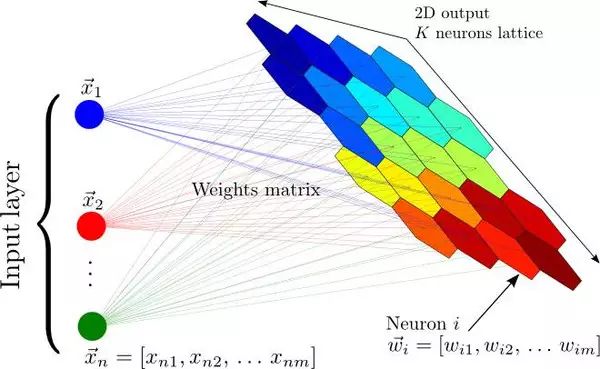
Self-organizing map neural network: mapping a large input vector to a grid of neural outputs, where each output is a cluster. Adjacent neurons represent the same cluster.
As with weight sharing, the earliest discussions about autoencoders were made in the aforementioned 1986 analysis of backpropagation. With weight sharing, it resurfaced in more research in the following years, including Hinton himself. This paper has an interesting title: “Autoencoders, Minimum Description Length, and Helmholtz Free Energy,” proposing that “the most natural method of unsupervised learning is to use a model that defines a probability distribution rather than observable vectors,” and using a neural network to learn such a model. So, there is another wonderful thing you can do with neural networks: approximate probability distributions.
Neural Networks Welcome Belief Networks
In fact, before becoming a co-author of the influential 1986 paper discussing the backpropagation learning algorithm, Hinton was studying a neural network method that could learn the probability distributions in “A Learning Algorithm for Boltzmann Machines” from 1985.
Boltzmann machines are networks similar to neural networks and have units very similar to perceptrons, but these machines do not compute output based on inputs and weights; given the values of connected units and weights, each unit in the network can compute its own probability, yielding a value of either 1 or 0. Thus, these units are random—they follow a probability distribution rather than a known deterministic manner. The Boltzmann part relates to probability distributions, which need to consider the states of particles in the system, which are themselves based on the energy of the particles and the thermodynamic temperature of the system. This distribution not only determines the mathematical methods of the Boltzmann machine but also dictates its reasoning methods—the units in the network have energy and states, and learning is accomplished by minimizing system energy and thermodynamic stimulation directly. Although not very intuitive, this energy-based reasoning deduction is actually an instance of an energy-based model and can be applied to an energy-based learning theoretical framework, in which many learning algorithms can be expressed.

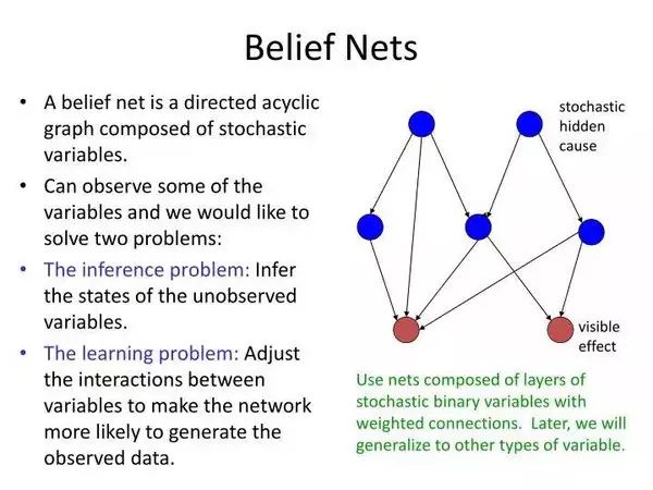
A simple belief, or Bayesian network—Boltzmann machines are essentially like this, but with non-direct/symmetric connections and trainable weights that can learn probabilities under specific patterns.
Returning to Boltzmann machines. When such units are placed together in a network, they form a graph, and data graphical models are similar. Essentially, they can do some very similar things to ordinary neural networks: certain hidden units compute the probabilities of certain hidden variables given known values of visible units representing observable variables (input—image pixels, text characters, etc.). For example, in classifying digit images, the hidden variable is the actual digit value, while the visible variable is the image’s pixels; given the digit image “1” as input, the values of the visible units can be known, and the hidden units model the probability that the image represents “1,” which should yield a higher output probability.
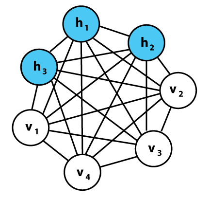
Instances of Boltzmann machines. Each row has associated weights, just like a neural network. Note that there is no hierarchy here—all things may be related to each other.
Thus, for classification tasks, there is now a good way to compute the probabilities of each category. This is very similar to the actual output calculation process of normal classification neural networks, but these networks have another little trick: they can produce seemingly reasonable input data. This is derived from the relevant probability equations—networks not only learn to compute the probabilities of hidden variable values when known visible variable values are given, but they can also infer the probabilities of visible variable values from known hidden variable values. So, if we want to derive an image of the digit “1,” the units associated with the pixel variables know they need to output a probability of 1, and the image can be derived based on probability—these networks will recreate image models. While it may achieve goals very similar to supervised learning of ordinary neural networks, the unsupervised learning task of learning a good generative model—probabilistically learning some hidden structures of the data—is generally required by these networks. Most of this is not fiction; learning algorithms do exist, and the special formulas that make this possible are as described in their papers:
Perhaps the most interesting aspect of the Boltzmann machine formula is that it can lead to a (domain-independent) general learning algorithm that modifies the connection strengths between units in a way that develops an internal model of the entire network (this model can capture the underlying structure of its environment). There has been a long history of failed attempts to find such an algorithm (Newell, 1982), and many people (especially in the field of artificial intelligence) now believe that no such algorithm exists.
We will not delve into all the details of the algorithm; we will just list some highlights: it is a variant of the maximum likelihood algorithm, which simply means it seeks to maximize the probability of the network’s visible unit values matching known correct values. Calculating each unit’s most likely actual value requires high computational demand; thus, training Gibbs sampling—starting with a random unit value network and continuously iterating to reassign values to units given the connection values—was used to provide some actual known values. When learning with the training set, visible unit values are set to obtain the current training sample’s values, thus hidden unit values are obtained through sampling. Once some true values are extracted, we can adopt a method similar to backpropagation—calculating the derivative for each weight value and estimating how to adjust the weights to increase the probability of the entire network making correct predictions.
Like neural networks, the algorithm can be performed in both supervised (knowing hidden unit values) and unsupervised ways. Although this algorithm has proven effective (especially when facing the “encoding” problem solved by autoencoder neural networks), it quickly became apparent that it was not particularly efficient. Redford M. Neal’s 1992 paper “Connectionist learning of belief networks” demonstrated the need for a faster method, stating: “These capabilities make Boltzmann machines very attractive in many applications—if not for the learning process, which is usually considered painfully slow.” Therefore, Neal introduced the idea of belief networks, which essentially resemble Boltzmann machines controlling and sending connections (thus introducing layers, just like the neural networks we saw earlier, rather than the above Boltzmann machine control concept). Stepping away from the tedious probability mathematics, this change allowed the network to be trained with a faster learning algorithm. The sprinkler and rain layer above can be viewed as having a belief network—this term is very rigorous because this probability-based model, in addition to being related to the field of machine learning, also has a close connection with the field of probability in mathematics.
Although this method is an improvement over the Boltzmann machine, it is still too slow; the mathematical demands of correctly calculating the probability relationships between variables are too large, and there are no simplification techniques yet. Hinton, Neal, and two other collaborators quickly proposed some new techniques in their 1995 paper “The wake-sleep algorithm for unsupervised neural networks.” This time, they produced a network somewhat different from the previous belief network, now called the “Helmholtz machine.” Without discussing the details again, the core idea is to take two sets of different weights for estimating hidden variables and generating calculations for known variables, the former called recognition weights and the latter generative weights, retaining the directional characteristics of Neal’s belief network. This way, when applied to the supervised and unsupervised learning problems of Boltzmann machines, training becomes much faster.
Ultimately, training belief networks will be somewhat faster! Although it did not have a significant impact, this algorithm improvement is a very important advancement for unsupervised learning of belief networks, comparable to the breakthroughs of backpropagation a decade ago. However, so far, new machine learning methods have also begun to emerge, and people have started to question neural networks because many of the ideas seem based on intuition, and because computers still struggle to meet their computational demands. As we will see in the third part, the winter of artificial intelligence will arrive in a few years. (To be continued)
Kurt Hornik, Maxwell Stinchcombe, Halbert White, Multilayer feedforward networks are universal approximators, Neural Networks, Volume 2, Issue 5, 1989, Pages 359-366, ISSN 0893-6080, http://dx.doi.org/10.1016/0893-6080(89)90020-8.
LeCun, Y; Boser, B; Denker, J; Henderson, D; Howard, R; Hubbard, W; Jackel, L, “Backpropagation Applied to Handwritten Zip Code Recognition,” in Neural Computation , vol.1, no.4, pp.541-551, Dec. 1989 89
D. E. Rumelhart, G. E. Hinton, and R. J. Williams. 1986. Learning internal representations by error propagation. In Parallel distributed processing: explorations in the microstructure of cognition, vol. 1, David E. Rumelhart, James L. McClelland, and CORPORATE PDP Research Group (Eds.). MIT Press, Cambridge, MA, USA 318-362
Fukushima, K. (1980), ‘Neocognitron: A Self-Organizing Neural Network Model for a Mechanism of Pattern Recognition Unaffected by Shift in Position’, Biological Cybernetics 36 , 193–202 .
Gregory Piatetsky, ‘KDnuggets Exclusive: Interview with Yann LeCun, Deep Learning Expert, Director of Facebook AI Lab’ Feb 20, 2014. http://www.kdnuggets.com/2014/02/exclusive-yann-lecun-deep-learning-facebook-ai-lab.html
Teuvo Kohonen. 1988. Self-organized formation of topologically correct feature maps. In Neurocomputing: foundations of research, James A. Anderson and Edward Rosenfeld (Eds.). MIT Press, Cambridge, MA, USA 509-521.
Gail A. Carpenter and Stephen Grossberg. 1988. The ART of Adaptive Pattern Recognition by a Self-Organizing Neural Network. Computer 21, 3 (March 1988), 77-88.
H. Bourlard and Y. Kamp. 1988. Auto-association by multilayer perceptrons and singular value decomposition. Biol. Cybern. 59, 4-5 (September 1988), 291-294.
P. Baldi and K. Hornik. 1989. Neural networks and principal component analysis: learning from examples without local minima. Neural Netw. 2, 1 (January 1989), 53-58.
Hinton, G. E. & Zemel, R. S. (1993), Autoencoders, Minimum Description Length and Helmholtz Free Energy., in Jack D. Cowan; Gerald Tesauro & Joshua Alspector, ed., ‘NIPS’ , Morgan Kaufmann, , pp. 3-10 .
Ackley, D. H., Hinton, G. E., & Sejnowski, T. J. (1985). A learning algorithm for boltzmann machines*. Cognitive science, 9(1), 147-169.
LeCun, Y., Chopra, S., Hadsell, R., Ranzato, M., & Huang, F. (2006). A tutorial on energy-based learning. Predicting structured data, 1, 0.
Neal, R. M. (1992). Connectionist learning of belief networks. Artificial intelligence, 56(1), 71-113.
Hinton, G. E., Dayan, P., Frey, B. J., & Neal, R. M. (1995). The” wake-sleep” algorithm for unsupervised neural networks. Science, 268(5214), 1158-1161.
Dayan, P., Hinton, G. E., Neal, R. M., & Zemel, R. S. (1995). The helmholtz machine. Neural computation, 7(5), 889-904.
Reprinted from Algorithms and the Beauty of Mathematics