Introduction
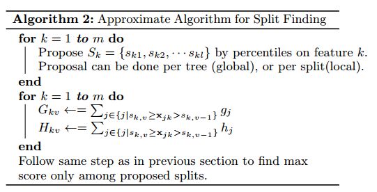
The previous article introduced the algorithm principles of XGBoost and introduced the scoring function (objective function) that measures the quality of tree structures. The best split point is selected based on the scoring function before and after the feature split points, but a detailed introduction to the node splitting algorithm was not provided. This article provides a detailed introduction to the split point algorithm of XGBoost, referencing Dr. Tianqi Chen’s paper “XGBoost: A Scalable Tree Boosting System”. Reply with XGBoost to get the paper download link.
Table of Contents
-
Parallel Principle
-
Greedy Algorithm for Split Point
-
Quantile Algorithm for Split Point
-
Weighted Quantile Algorithm for Split Point
-
Splitting Algorithm for Sparse Data
-
Conclusion
1. Parallel Principle
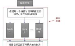
XGBoost generates CART trees serially, but it can process features in parallel. The parallel principle of XGBoost is reflected in the selection of the optimal split point. Suppose there are M features in the sample data; the best split point algorithm in the process of constructing a CART tree is as follows:
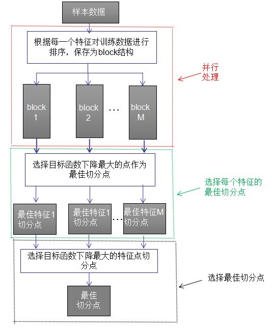
1. The red box indicates sorting the training data according to the size of each feature and saving it as a block structure, with the number of blocks equal to the number of features.
2. The green bar indicates selecting the best feature split point for each block structure, where the node splitting criterion is the degree of decrease of the objective function, which can be referenced in the previous text.
3. The black box indicates comparing the gains of the objective function decrease for the best feature split points of each block structure and selecting the best split point.
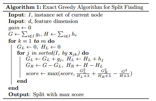
2. Greedy Algorithm for Split Point
The splitting point algorithm for each block structure follows the same idea; therefore, I will focus on the splitting point algorithm for a specific block structure.
XGBoost quantile algorithm: Sort the sample data based on features, then split the features from small to large, compare the objective function’s value after each split, and select the node with the maximum decrease as the optimal split point for that feature. Finally, compare the objective function decrease values of the optimal split points from different block structures and select the feature with the maximum decrease as the optimal split point.
The flowchart is as follows:
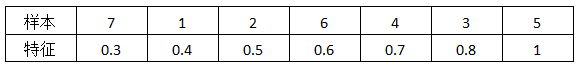
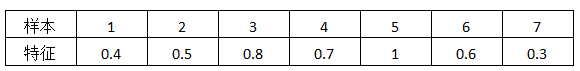
[Example] The table below shows the feature values of a certain column in the samples.

Re-sort the samples based on feature size:
Greedy algorithm split nodes:
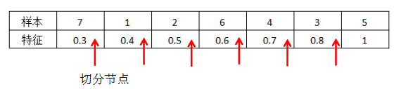
The red arrows indicate each split node, selecting the point where the objective function decreases the most as the split node.
3. Quantile Algorithm for Split Point
If the feature is a continuous value, the computation using the above greedy algorithm is extremely large. When the sample size is sufficiently large, use feature quantiles to split features. The flowchart is as follows:
[Example] The table below shows the feature values of a certain column in the samples, using the third quantile as the split node.
Sort the samples based on feature size:

Use the feature’s third quantile as the split node:
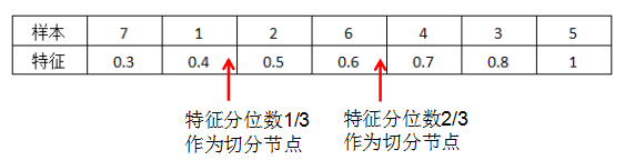
The red arrows indicate each split node, selecting the point where the objective function decreases the most as the split node.
4. Weighted Quantile Algorithm for Split Point
The previous section assumed equal sample weights. Using sample quantiles to evenly distribute the loss function introduces bias. This section uses sample weights to evenly distribute the loss function.
The loss function is as follows:
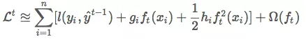
Transforming it gives:

The xi loss function can be viewed as the mean squared error with a label of −gi/hi, multiplied by the weight of size hi. In other words, the contribution weight of xi to the loss is hi, and the quantile of the sample weight equals the evenly distributed error.
The previous section assumed equal sample weights, using the quantile of feature values as the split point. This section assumes sample weights as hi, and the steps for constructing the evenly distributed sample weight are:
(1) Sort the samples based on feature size.
(2) Define the sorting function:
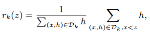
Where x and z represent features.
(3) Set the quantile of the sorting function as the split point.
[Example] See the figure below:

The relationship between features and corresponding sorting function values is shown in the table below:
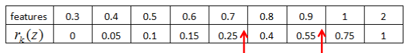
The red arrow indicates using the third quantile as the split point.
Finally, select the optimal split point.
5. Splitting Algorithm for Sparse Data
Sparse data is very common in practical projects, mainly caused by: 1. Missing data; 2. Statistical zeros; 3. One-hot encoded feature representations.
The splitting point algorithm for sparse data:

When feature values are missing, samples containing missing feature values are mapped to the default direction branch, and then the optimal split point for that node is calculated. The optimal split point corresponds to the default split direction when feature values are missing.
6. Conclusion
This article is the author’s understanding of Dr. Tianqi Chen’s paper “XGBoost: A Scalable Tree Boosting System”. If there are different opinions, feel free to communicate.
References:
Chen Tianqi “XGBoost: A Scalable Tree Boosting System”
Recommended Reading Articles
Summary of XGBoost Algorithm Principles

-END-