Machine Learning and Bioinformatics: XGBoost Analysis

With the continuous development of genetics, breeding, and the increasing advancements in the Human Genome Project and molecular biology, biological data has experienced explosive growth over just a few decades. For example, algorithms such as regression analysis, random forests, and support vector machines in bioinformatics are already quite mature. Recently, while reading literature, I came across a paper in materials science that utilized the XGBoost algorithm, which is very similar to the algorithms I previously studied in two bioinformatics articles. Today, let’s analyze what sparks may arise when bioinformatics meets machine learning, and how to integrate these interesting machine learning methods into your own articles to increase innovation and help reduce costs when submitting purely analytical papers.

1. Bioinformatics Data

The types of data studied can be divided into genotype data and expression data; among them, genotype data is obtained through WGS, WES, and gene chip data.

2. The Combination of Machine Learning and Bioinformatics Data

We increasingly see the application of machine learning in bioinformatics articles, for example, finding usable patterns from data and then making predictions. Typically, these predictive models are used in operational processes to optimize decision-making, but they can also provide critical insights and information for reporting strategic decisions.

The basic premise of machine learning is algorithm training, predicting output values within a certain probability range when specific input data is provided. Remember that the trick of machine learning is induction rather than deduction—related to probability, not a final conclusion.

The process of building these algorithms is called predictive modeling. Once this model is mastered, sometimes it can be directly applied to analyze raw data and predict certain important information in new data. The output of the model can be classifications, possible outcomes, hidden relationships, attributes, or estimates.

If we are concerned with estimated values or continuous values, predictions can also be represented numerically. The type of output determines the best learning method and will affect the metrics we use to judge model quality.

Who supervises machine learning methods? Machine learning methods can be either supervised or unsupervised. The distinction is not whether the algorithm can do as it pleases, but whether it learns from training data with real results—pre-determined and added to the dataset to provide supervision—or attempts to discover any natural patterns within a given dataset. Most businesses use predictive models, employing supervised methods on training data, and are usually aimed at predicting whether a given instance—email, person, company, or transaction—belongs to an interesting category—spam, potential buyer, creditworthy, or obtaining follow-up quotes.

If you are not very clear about what you are looking for before starting, then unsupervised machine learning methods can provide fresh insights. Unsupervised learning can also generate clusters and hierarchical graphs, showing the intrinsic relationships of the data, and can discover which data fields appear to be independent, and which are rule descriptions, summaries, or generalizations. In turn, these insights can aid in building better predictive methods.

Building machine learning models is a repetitive process that requires data cleaning and hands-on experimentation. Currently, some automated and guided modeling tools are emerging in the market, promising to reduce dependence on data scientists while achieving the highest return on investment in common areas. However, the real difference in here is likely something you will need to discover yourself.

With the development of deep learning technologies, autoencoders are used to integrate multi-omics data and extract representative features. However, due to the impact of data noise, the generated models can be fragile. Additionally, previous studies often focused on single cancer types, without comprehensive testing across pan-cancer.

3. Algorithm Introduction

1. GBDT (Gradient Boosting Decision Tree):It performs well in data analysis and prediction. It is an ensemble algorithm based on decision trees.

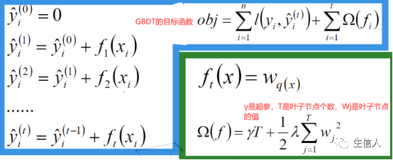
2. Boosting:Boosting refers to adding multiple weak learners to produce a new strong learner. Classic examples include: AdaBoost, GBDT, XGBoost, etc. If each weak learner is represented by

Machine Learning and Bioinformatics: XGBoost Analysis

, then the strong learner of Boosting can be represented as:

In simple terms, it is equivalent to chaining multiple learners (bagging is parallel). Next, we will introduce the XGBoost algorithm.

3. XGBoost:XGBoost is essentially a GBDT, but strives to maximize speed and efficiency, hence the name X (Extreme) GBoosted.

XGBoost Tree Definition:

Example

Predicting a family’s preference for lipstick, considering that younger people are more likely to like lipstick compared to older individuals, and females are more likely to like lipstick than males. Therefore, we first differentiate between adults and minors based on age, and then distinguish between males and females based on gender, scoring each individual’s preference for lipstick, as shown in the figure below.

The core algorithm of XGBoost is not difficult, basically:

1. Continuously add trees and perform feature splits to grow a tree. Each time a tree is added, it actually learns a new function f(x) to fit the residuals predicted from the last iteration.

2. Once we have trained k trees, to predict the score of a sample, we actually determine which leaf node the sample’s features will fall into in each tree, with each leaf node corresponding to a score.

3. Finally, we just need to sum the scores corresponding to each tree to get the predicted value for that sample.

In simple terms, XGBoost is an improvement of the GBDT algorithm, a commonly used supervised ensemble learning algorithm; it is a scalable and convenient Gradient Boosting algorithm that can be built in parallel.

The principle is: adding a penalty term on the basis of the GBDT objective function, reducing model complexity by limiting the number of leaf nodes in the tree model and the values of the leaf nodes to prevent overfitting. The division by two is for convenience in derivation. t is the number of trees, and obj is the loss function.

(If you don’t understand, that’s okay, just grasp the purpose of doing this~ The general steps are to prevent overfitting, the second-order Taylor expansion formula calculation provides a new tree division standard using the incremental of the loss function).

Purpose: To find out how the t-th tree is constructed, so our expectation is that the loss function only relates to the t-th tree.

XGBoost appeared relatively early, but its application in interdisciplinary fields such as biology, chemistry, and materials is relatively scarce. Capturing this novel direction may add highlights to your paper. XGBoost supports development languages: Python, R, Java, Scala, C++, etc.

The best source of information for XGBoost is the official GitHub repository of the project: https://github.com/dmlc/xgboost.

4. Literature and Summary

First Paper: “Improving protein-protein interactions prediction accuracy using XGBoost feature selection and stacked ensemble classifier”

Machine Learning and Bioinformatics: XGBoost Analysis

Journal: “Computers in Biology and Medicine”

Impact Factor and CAS Division: IF: 3.434, CAS Division 3

Publication Date: July 2020

Author Unit: Qingdao University of Science and Technology

1. Algorithm Method

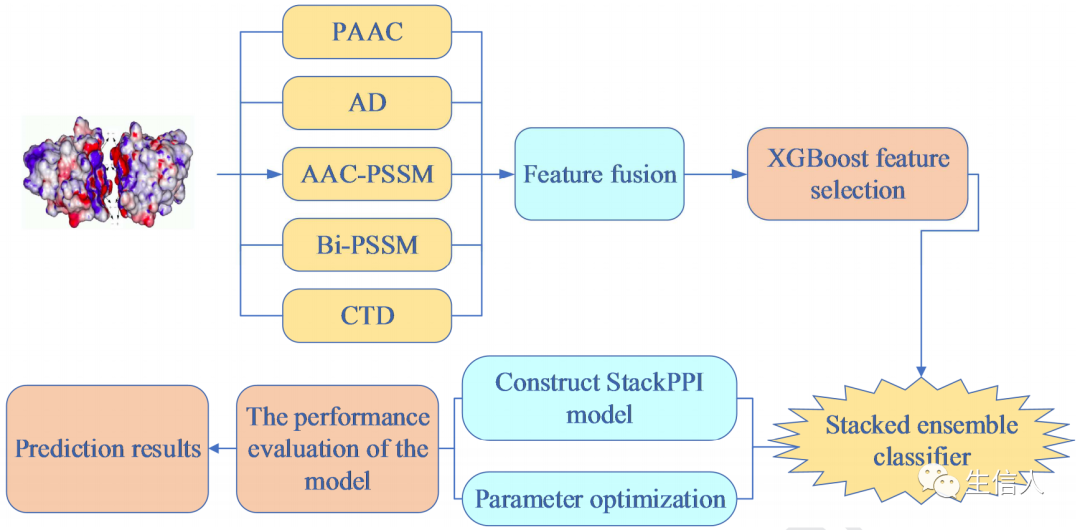
(1) The authors proposed a new method for predicting protein-protein interactions—StackPPI.

(2) Fusion of PAAC, AD, AAC-PSSM, Bi-PSSM, and CTD to extract physicochemical, evolutionary, and sequence information.

(3) XGBoost feature selection method is used to eliminate redundancy and retain the optimal subset of features.

(4) For the first time, a stacked ensemble classifier was constructed using RF, ET, and LR.

2. Data

Training Set:

Helicobacter pylori, with 1458 positive and negative samples each.

Saccharomyces cerevisiae, with 5594 positive and negative samples each.

Test Set:

Human interaction pairs: 1412

Mouse interaction pairs: 313

C. elegans interaction pairs: 4013

E. coli interaction pairs: 6954

Gene evaluation dataset:

Wnt-related pathway: 96 interactions

Diseases specificity: 108 interactions

3. Result Interpretation:

Flowchart:

Machine Learning and Bioinformatics: XGBoost Analysis

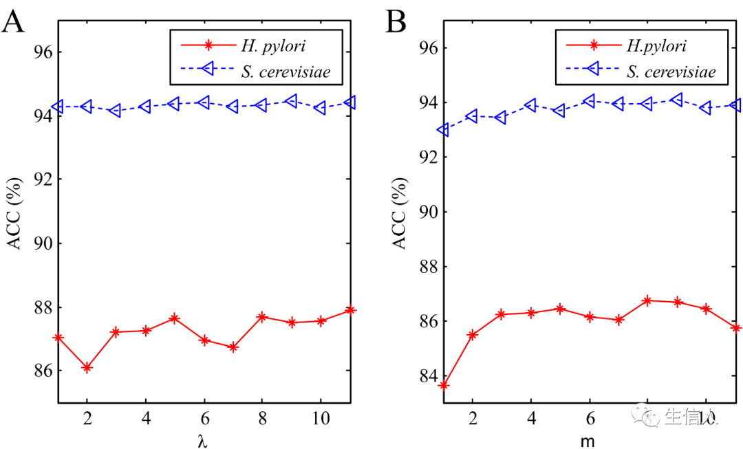
(1) Determining parameter m.

Machine Learning and Bioinformatics: XGBoost Analysis

As shown in Figure 2 (A), with the change of parameter λ, the ACC values of the two datasets are different. When λ=11, the accuracy (ACC) of StackPPI reaches a global maximum on both the Helicobacter pylori and yeast datasets, while on the Helicobacter pylori dataset, it reaches a maximum when λ=9. Using average accuracy, the optimal parameter λ for PAAC in StackPPI (λ=11) is obtained. Figure 2 (B) shows the changes in ACC of Moreau-Broto, Moran, and Geary autocorrelation descriptors under different m values. The highest ACC for Helicobacter pylori is at m=8, while for yeast StackPPI it is highest at m=9. By average predictive accuracy, set m=9 in StackPPI, the dimensionality of the autocorrelation descriptor AD (Moreau-Broto, Moran, and Geary, amino acid composition position-specific scoring matrix) is 21*9=189.

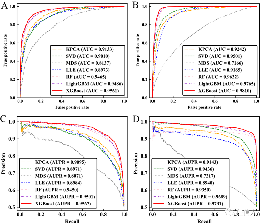
(2) Assessment and selection of dimensionality reduction methods.

Machine Learning and Bioinformatics: XGBoost Analysis

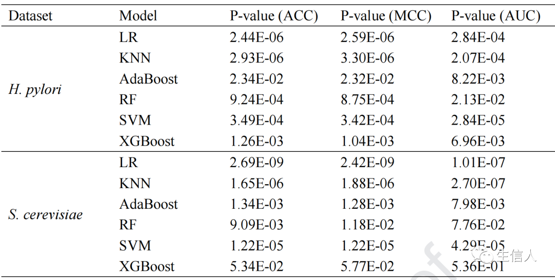
For different datasets, different methods are used, and effectiveness is assessed through the receiver operating characteristic curve. To select the optimal classification algorithm, the stacked ensemble classifier is compared with logistic regression (LR), k-nearest neighbors (KNN), AdaBoost, random forests (RF), support vector machines (SVM), and XGBoost. Among them, the neighborhood for the KNN method is set to 5, SVM uses radial basis kernel, and the ‘n_estimators’ for AdaBoost, RF, and XGBoost are set to 500, 500, and 500 respectively. Therefore, in this section, XGBoost is used as the classifier. To further validate StackPPI, the authors conducted statistical tests on different classifiers. The p-values of LR, KNN, AdaBoost, RF, SVM, and XGBoost compared to the stacked ensemble classifier are reported for ACC, MCC, and AUC metrics.

Machine Learning and Bioinformatics: XGBoost Analysis

4. Summary: Protein-protein interactions (PPIs) participate in most cellular activities at the proteomic level. In this article, the authors explore and predict protein interactions using machine learning algorithms combined with bioinformatics data. The authors propose a prediction framework called StackPPI. First, pseudo-amino acid composition, autocorrelation descriptors (Moreau-Broto, Moran, and Geary, amino acid composition position-specific scoring matrix), bi-gram position-specific scoring matrix, and composition, transition, and distribution are used to encode biologically relevant features. Secondly, the XGBoost algorithm is used to eliminate feature noise and perform dimensionality reduction through gradient boosting and average gain; finally, the optimized features are analyzed through StackPPI (a PPI predictor developed from a stacked ensemble classifier composed of random forests, extremely randomized trees, and logistic regression algorithms).

Second Paper: “Integrating multi-omics data through deep learning for accurate cancer prognosis prediction”

Machine Learning and Bioinformatics: XGBoost Analysis

Journal: “Computers in Biology and Medicine”

Impact Factor and CAS Division: IF: 3.434, CAS Division 3

Publication Date: May 2021

Author Unit: Sun Yat-sen University

1. Algorithm Method:

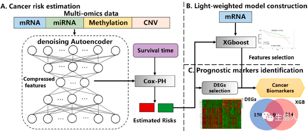
(1) The architecture of the DCAP method: High-dimensional features of multi-omics cancer data are input into the DAE network to obtain representative features, which are then used to estimate patient risk through the Cox model. Considering that it is clinically difficult to obtain multi-omics data, the authors further constructed an XGBoost model using mRNA data to fit the estimated risk. The constructed model is used to predict the risk of cancer patients in independent datasets. Furthermore, based on genes identified through XGBoost and differential expression analysis, the authors identified 9 prognostic markers highly related to breast cancer prognosis.

(2) Autoencoder

(3) XGBoost features to create risk models,

2. Data:

(1) TCGA cancer data

(2) GEO cancer data

3. Result Interpretation:

Flowchart:

Machine Learning and Bioinformatics: XGBoost Analysis

(1) Comparison and selection of data types and methods.

Machine Learning and Bioinformatics: XGBoost Analysis

As shown in Table 2, DCAP achieved nearly the same c-index values in 10-fold CV and independent validation, with averages of 0.678 and 0.665 for 15 types of cancer, respectively. The results indicate that the method has good robustness. We further detail the contribution of each omics type in DCAP.

Machine Learning and Bioinformatics: XGBoost Analysis

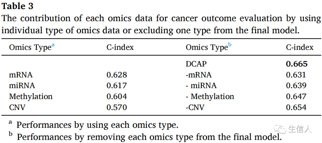
As shown in Table 3, among single omics data, mRNA performs the best with an average c-index of 0.628, while CNV performs the worst with a c-index of 0.570. miRNA and methylation rank second and third respectively. It is consistently observed that when excluding one omics type from DCAP, the c-index value caused by excluding mRNA decreases the most, from 0.665 to 0.631, while excluding CNV causes the smallest decrease in c-index. These results indicate that mRNA plays the most crucial role in identifying high-risk patients, while CNV has the least impact. On average, the prognostic prediction using multi-omics improves by 5.9% compared to using only mRNA data.

(2) Case Study

As a case study, the researchers applied the authors’ method to breast cancer (BRCA), which has the most samples. To validate the breast cancer prognosis prediction model constructed by DCAP-XGB, tests were conducted on three external breast cancer datasets GSE2990, GSE9195, and GSE17705 collected from the GEO database.

Machine Learning and Bioinformatics: XGBoost Analysis

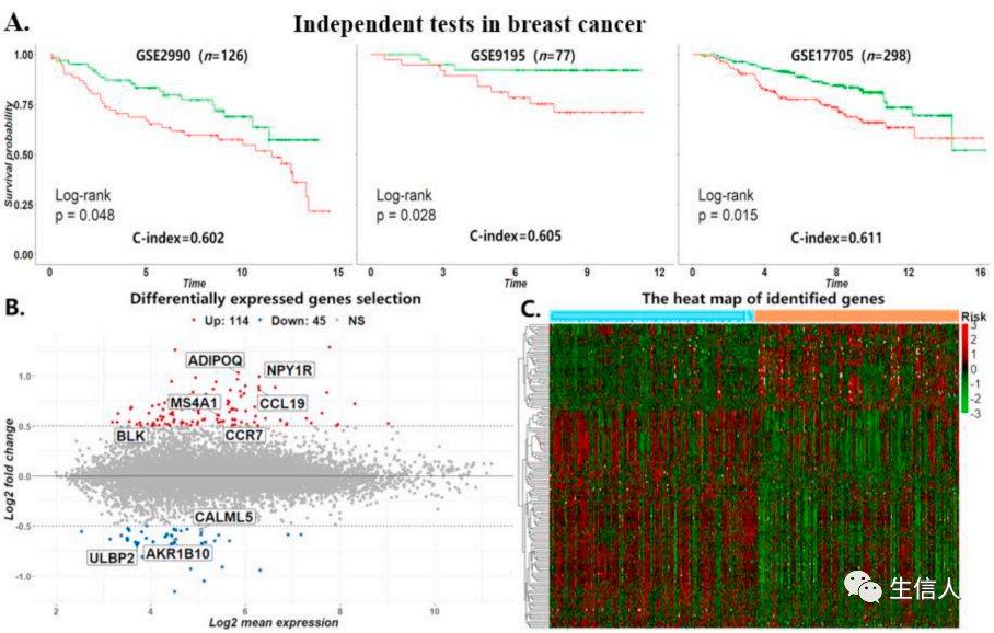
As shown in Figure 3A, the high-risk and low-risk groups predicted by the three datasets are clearly separated by survival curves, with p-values all below 0.05, and c-indices being similar (0.602, 0.605, 0.611). These results demonstrate the robustness of the authors’ lightly weighted risk prediction model.

Based on the DCAP classification of high-risk and low-risk populations, we identified 159 DEGs, of which 45 risk genes were downregulated and 114 risk genes were upregulated (Figure 3B). Among the 159 DEGs, 57 (35.9%) genes have been confirmed in the literature to be associated with breast cancer.

Using the 223 genes selected by the XGBoost model, we found 9 overlapping DEGs, of which 7 (77.8%) genes (ADIPOQ, NPY1R, CCL19, MS4A1, CCR7, CALML5, and AKR1B10) are associated with breast cancer (Table 5). For the remaining 2 genes (ULBP2 and BLK), although there is no direct literature proving their association with breast cancer prognosis, it has been reported that the induction of ULBP2 is related to the pharmacological activation of p53 triggering an anti-cancer innate immune response, while BLK is a true oncogene suitable for studying BLK-driven lymphoma and screening new BLK inhibitors in vivo.

4. Summary:

Today, genomic information is widely used for precision treatment of cancer. Since the omics data of individual types only represent a single perspective, there is data noise and bias; therefore, various types of omics data are needed to accurately predict cancer prognosis. However, due to the presence of a large number of redundant variables in multi-omics data, while the sample size is relatively small, effectively integrating multi-omics data poses certain challenges. With the development of deep learning technology, autoencoders are used to obtain robust representations of multi-omics data, and then use the learned representative features to estimate patient risk. Applying samples from 15 cancer types in the American Cancer Genome Atlas (TCGA), the results show that this method improves average performance by 6.5% compared to traditional methods. Considering the practical difficulty of obtaining multi-omics data, the authors further trained an XGBoost model, fitting the estimated risk using only mRNA data, and found that the model had an average c-index of 0.627. Taking the breast cancer prognosis prediction model as an example, independent tests were conducted on three datasets from the Gene Expression Omnibus (GEO), and the results showed that the model could significantly distinguish between high-risk and low-risk patients. Based on the risk subgroups classified by the authors’ method, 9 prognostic markers highly associated with breast cancer were identified, of which 7 genes have been confirmed by literature review. Thus, it can be concluded that this study constructed an accurate and robust framework for predicting tumor prognosis based on integrated multi-omics data. Additionally, it serves as an effective way to discover cancer prognosis-related genes.

Third Paper: “XGBoost model for electrocaloric temperature change prediction in ceramics”

Machine Learning and Bioinformatics: XGBoost Analysis

Journal: “npj Computational Materials” published by the Shanghai Institute of Silicate Research, Chinese Academy of Sciences

Impact Factor and CAS Division: IF: 12.3, CAS Division 1

Publication Date: July 2022

Author Unit: Carnegie Mellon University

1. Algorithm Method:

(1) XGBoost algorithm

2. Data:

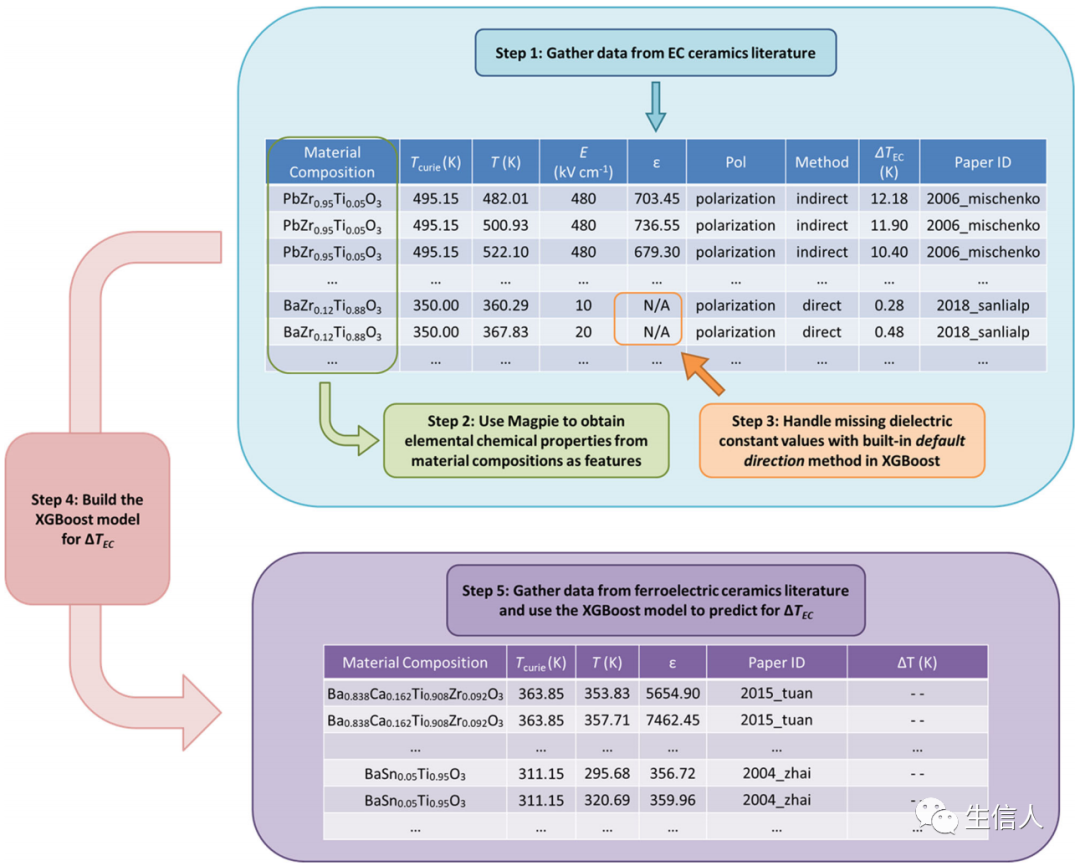
(1) Electrocaloric (EC) materials dataset: EC materials mainly fall into three categories: polymers, ceramics, and polymer-ceramic composites. The authors established a dataset for EC ceramics due to their diverse composition. The authors extracted information from existing literature, as most material compositions do not appear in well-known material databases. This dataset includes 97 materials from 45 papers and can be accessed in CSV format on GitHub. A snapshot of the dataset and a flowchart of the data collection and model building steps are shown below.

Machine Learning and Bioinformatics: XGBoost Analysis

3. Result Interpretation:

(1) Data preprocessing

Machine Learning and Bioinformatics: XGBoost Analysis

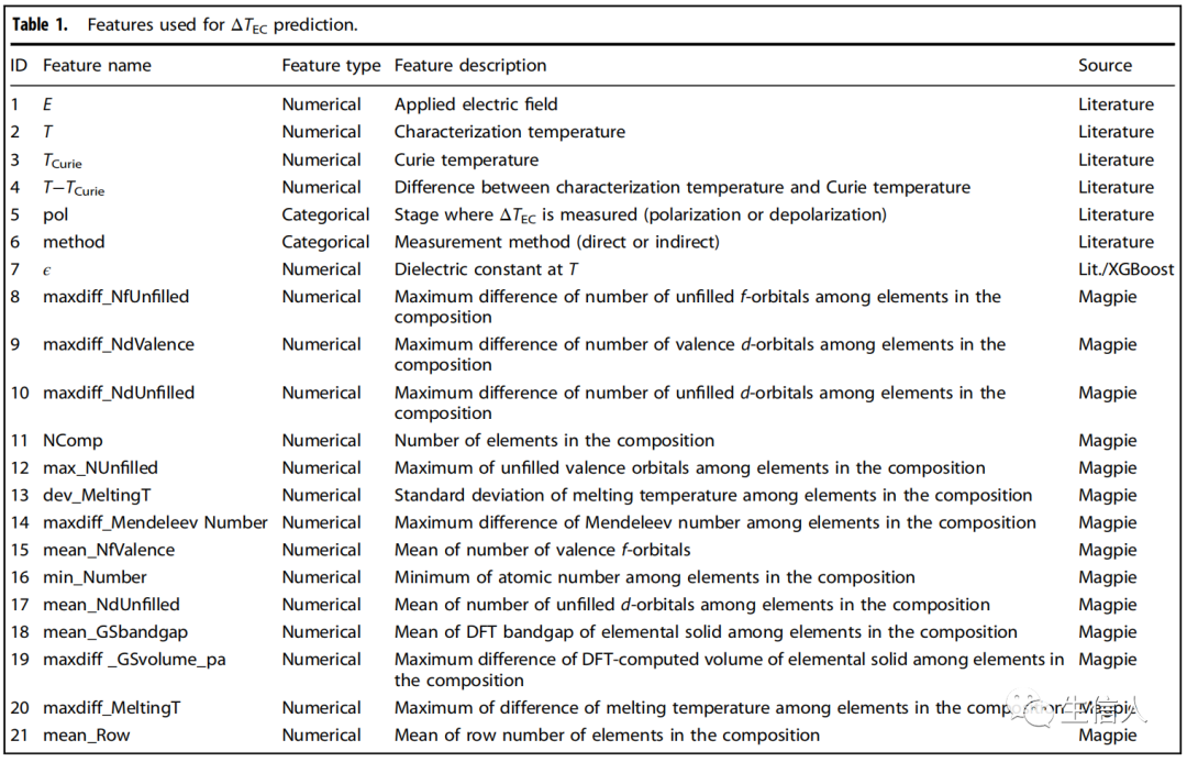
After some preprocessing steps to remove unqualified data, researchers had 4406 data points, each containing 21 features listed in Table 1 (7 experimental conditions/material properties features and 14 confounding features). The label to be predicted is ΔTEC under given conditions (i.e., T and E).

Machine Learning and Bioinformatics: XGBoost Analysis

In Figure 2a, the collected data is plotted as a function of temperature at full scale characterization. In Figure 2b, data points of ΔTEC within the 0-2k range are plotted as a function of T-TCurie. Different colors represent different material compositions, and the size of the markers is proportional to the applied electric field. The temperature changes of these EC materials are relatively small, with a median of 0.36 K and an average of 1.07 K. Among the 97 materials, 3 have maximum values far exceeding the second-largest maximum value of 13 K. These three materials are marked as outliers and were excluded from model building unless otherwise specified.

(2) XGBoost modeling

Machine Learning and Bioinformatics: XGBoost Analysis

The XGBoost regression model used for ΔTEC prediction (see methods XGBoost regression section) was established through a grid search for the best hyperparameter set from 6912 combinations (Table 2). Since XGBoost cannot extrapolate, it can only make reasonable predictions on situations previously encountered in the training history; unless otherwise specified, the materials with the lowest and highest ΔTEC values will be forced to appear in the training set. The authors built three models, distinguished by their random seeds. Although, as expected, the XGBoost model cannot predict ΔTEC values higher than the maximum in the training set, they all have prediction capabilities for ΔTEC values of PbZr0.97La0.02(Zr0.95Ti0.05)O3 that exceed the maximum in the training set. This observation indicates that the XGBoost model learns from fundamental physics and can serve as a useful tool for qualitative predictions and improving the search for new materials.

(3) Model validation

Based on the distances of 94 EC ceramics in feature space, they were divided into training and testing datasets. First, the complex features of EC materials were projected into a two-dimensional t-distributed stochastic neighbor embedding (t-SNE) space. Then, k-means clustering was performed on the projections of the 94 materials. By plotting the within-cluster sum of squares as a function of k and identifying the “elbow”, the optimal k value was determined to be 3. A clustering label was assigned to all data. 75% of the materials from each cluster were selected as training data, while the remaining 25% were used for testing.

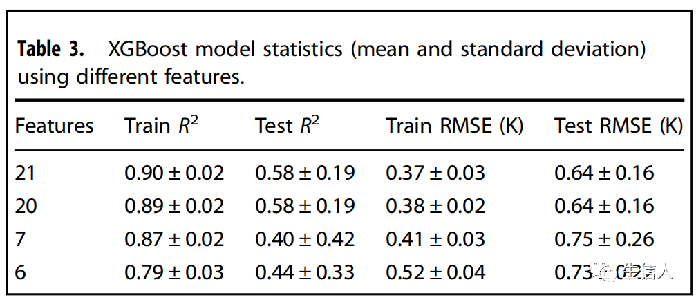
Different numbers of features were used to build models. These included 21 features listed in Table 1, 20 features excluding dielectric constant, 7 features excluding all confounding features, and features excluding dielectric constant and all confounding features. For each feature set, 100 XGBoost models were trained using the same hyperparameters but different random seeds and training/testing splits. The R2 and RMSE results (averages and standard deviations) are summarized in Table 3, where each row corresponds to 100 models.

Machine Learning and Bioinformatics: XGBoost Analysis

(3) Feature analysis of the model for impurities

We performed feature analysis for the XGBoost ΔTEC model, with its parity plot shown in Figure 3.

Machine Learning and Bioinformatics: XGBoost Analysis

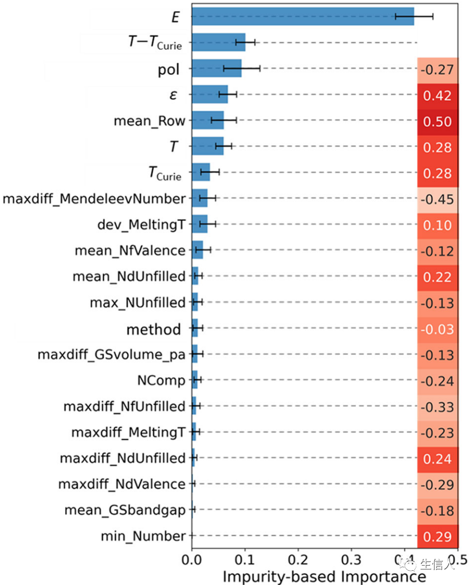
The impurity-based feature importance is calculated by XGBoost by measuring the total gain (i.e., improvement in accuracy) at all splits using the feature. The higher the feature importance value, the more important the feature is.

Machine Learning and Bioinformatics: XGBoost Analysis

The impurity-based feature importance is shown in Figure 4. The applied electric field E ranks first, followed by T-Tcurie. These observations are consistent with known physical properties. The 16 confounding features help the model distinguish different materials. Therefore, directly interpreting individual features may be challenging. The authors’ XGBoost model is strictly regularized (i.e., tree pruning and restrictions were used in node splits), and the model is not sensitive to the inclusion of irrelevant features. By using the XGBoost ΔTEC model for prediction, its parity plot is shown in Figure 3.

4. Summary:

XGBoost gradient boosting minimizes prediction errors through the gradient descent algorithm, producing a set of weak predictive models (in the form of decision trees). During training, gradient boosting adds a new regression tree each time to reduce residuals (i.e., the difference between model predictions and label values). The existing trees in the model remain unchanged, which slows down overfitting. In this study, the authors established an extreme gradient boosting (XGBoost) machine learning model to predict the electrocaloric (EC) temperature change of ceramics based on their composition (encoded by confounding element properties), dielectric constant, Curie temperature, and characterization conditions.

Based on experimental literature, a dataset of 97 EC ceramics was established. By sampling clustered data in feature space, the model achieved a coefficient of determination of 0.77 and a root mean square error of 0.38 K on the test data. Feature analysis indicates that the model captures known physical characteristics of effective conductivity materials. Confounding features help the model distinguish materials, with elemental electronegativity and ionic charge identified as key features. The model was applied to 66 uncharacterized ferroelectrics, identifying lead-free candidate materials with EC temperature changes greater than 2 K at room temperature and 100 kV/cm.

5. Article Summary

Genomics is an interdisciplinary biological science that quantifies all genes of an organism and studies their interactions and effects on the organism. Today, machine learning is widely applied in genomics research, using known training sets to predict outcomes of data types. Meanwhile, deep learning and deep learning models can predict and perform dimensionality reduction analysis more flexibly. With appropriate training data, deep learning can automatically learn features and patterns with minimal human intervention. Currently, deep learning has also been successfully applied to regulate genomics, mutation detection, and pathogenicity scoring, improving the interpretability of genomic data and transforming genomic data into actionable clinical information, improving disease diagnosis protocols, understanding who should use which drugs, and maximizing efficacy while minimizing drug side effects. Due to the numerous variables involved, manual statistical analysis is slow, while deep learning can help shorten the process.

XGBoost has extremely fast training speed, is memory-friendly, and can compute the importance of each feature, which is beneficial for feature selection, model interpretability, model transparency, and model tuning; XGBoost can also save tree models in plaintext format, facilitating model visualization and tuning. With so many advantages, hurry up and integrate it into your paper before it becomes widely used in the field of bioinformatics!

END

Don’t want to miss out on daily hot topics and technologies?

Welcome everyone to add Bioinformatics to your favorites.Starrecommendations

Written by ▎Dingr

Typeset by ▎CY.

Previous Recommendations

Character Specials

• Comprehensive summary of academician Dong Chen’s research results

• Series of research results by Professor Zhang Zemin

Immunity Specials

• Pure bioinformatics mining of immunotherapy in Division 2

• Multi-omics immunotherapy

Spatial Metabolism

• Single-cell sequencing combined with spatial transcriptomics

• Spatial metabolism + drug resistance

Iron Death Specials

• Summary of iron death articles

• Classic iron death, new ideas again

m6A Specials

• Integration of m6A regulatory factors in bioinformatics analysis

• Why does m6A glioma continue to rise?

Research Acceleration

• How bioinformatics accelerates research topics

• Essential skills for clinical research wet experiments

irAEs Specials

• irAEs: Overview

• irAEs: Bioinformatics signatures

For more bioinformatics analysis questions, consult: 18501230653 (WeChat same number)

Leave a Comment Cancel reply